SNT and Sholl Analysis are based on publications. Please cite them in your own research!
This page was last revised for version 5.0.0.
Please help us to keep up-to-date documentation by editing this page directly to fill in any documentation gap. Do reach out if you need assistance!
Automated Sholl for direct analysis of segmented images and traced morphologies. Features powerful quantifications based on curve fitting. Analysis of profiles obtained by other software is also possible.
Introduction
 The Sholl technique1 is used to describe neuronal arbors. SNT features a collection of tools that perform Sholl on reconstructed morphologies, or directly on 2D/3D images of isolated neurons (bypassing the need for reconstruction). The procedure is based upon how Sholl analysis is done by hand: Algorithms define a series of concentric shells (circles or spheroids) around a focal point of a neuronal arbor and count how many times the arbor intersects sampling shells. The major advantages of these tools over other implementations are:
- Both images and reconstructions can be analyzed
- When analyzing images directly, previous tracing of the arbor is not required
- Curve fitting is combined with several methods to automatically retrieve quantitative descriptors from sampled data, which allows direct statistical comparisons between arbors
- Continuous and repeated sampling around user-defined foci are allowed
- Angular, length-based, and intensity-based profiles
- Extensive options for quantitative analysis
- Batch processing is possible
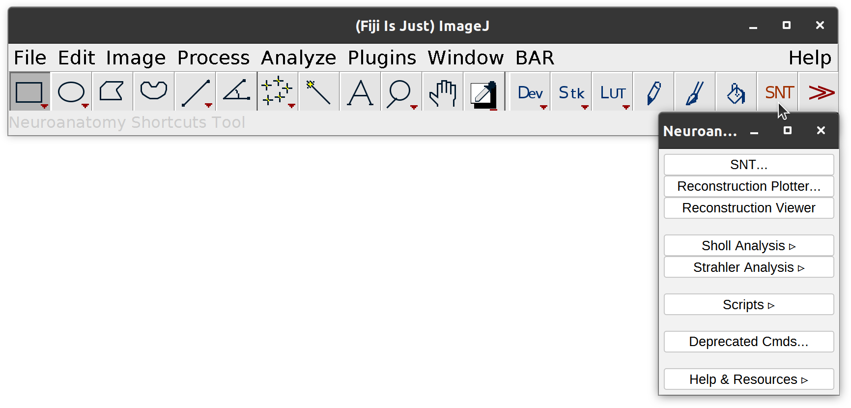
After installing SNT, Sholl commands can be accessed through the Plugins › Neuroanatomy › Neuroanatomy Shortcut Window (SNT icon in the ImageJ toolbar), or from SNT’s tracing interface.
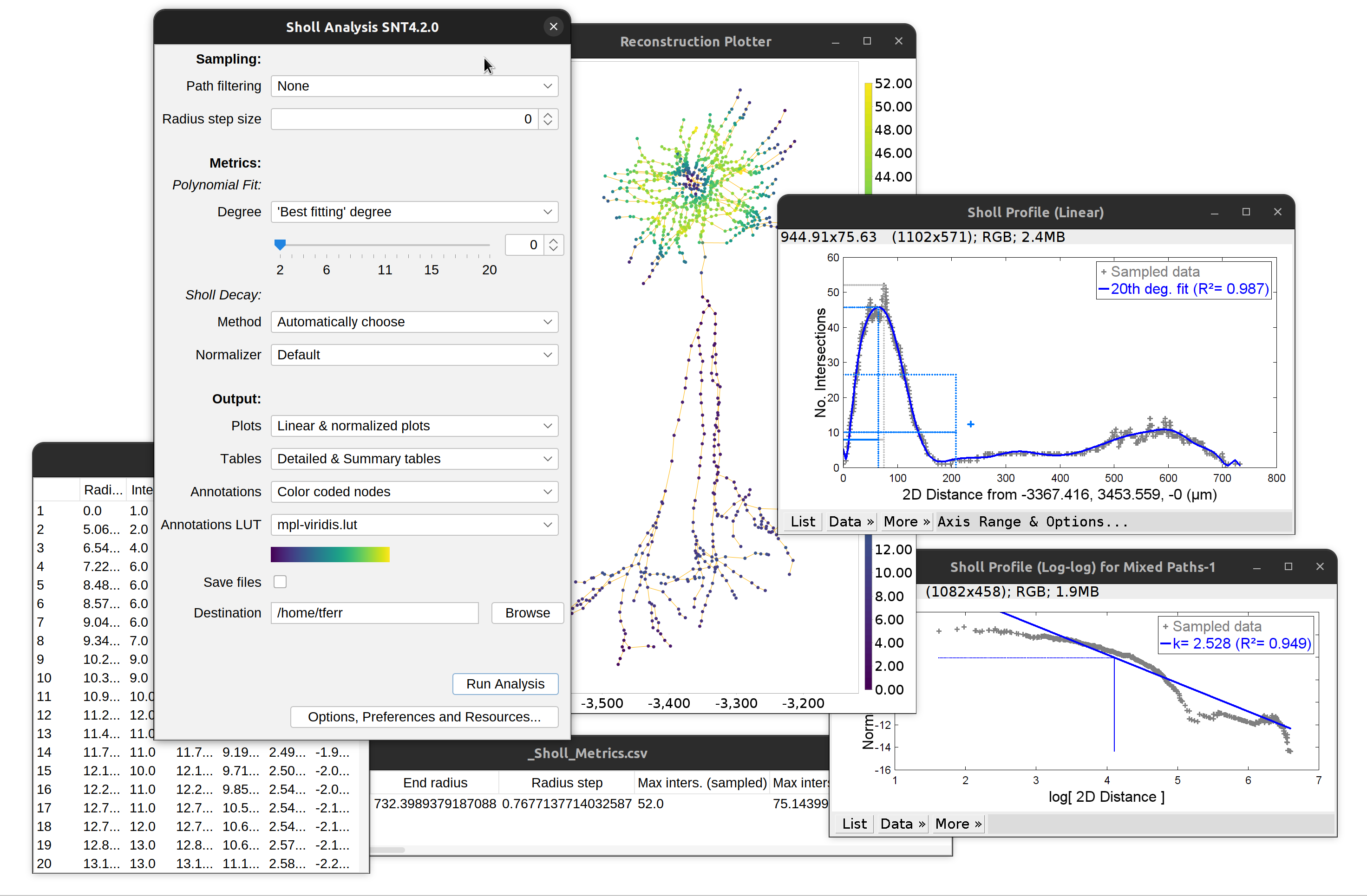 Overview of outputs: Linear and log-log profile (Sholl decay calculation), detailed and summary tables. ‘Traditional’ plots are obtained by disabling curve-fitting altogether
 hippocampal CA1 cell[^8] in which apical and basal dendrites have been analyzed [separately](#ca1-cell-plot) and [color coded](#output-options) according to their Sholl profile. Warmer hues indicate higher number of Intersections (*N*). [Critical radius](#critical-radius) (*r<sub>c</sub>*) and [Mean value](#mean-value-of-function) (*N<sub>av</sub>*) are indicated.](/media/plugins/snt/bitmapsholl-ca1mask.png) Skeletonized hippocampal CA1 cell2 in which apical and basal dendrites have been analyzed separately and color coded according to their Sholl profile. Warmer hues indicate higher number of Intersections (N). Critical radius (rc) and Mean value (Nav) are indicated.
Skeletonized hippocampal CA1 cell2 in which apical and basal dendrites have been analyzed separately and color coded according to their Sholl profile. Warmer hues indicate higher number of Intersections (N). Critical radius (rc) and Mean value (Nav) are indicated.
![Linear plot for the same CA1 cell[^8]. Using the soma as center, image was sampled twice using [hemishells](#hemishells) in order to segregate apical from basal dendrites. For clarity, distances for basal branches were assigned negative values and arbor overlaid (in green) over the profile.](/media/plugins/snt/bitmapsholl-ca1compartment.png) Linear plot for the same CA1 cell2. Using the soma as center, image was sampled twice using hemishells in order to segregate apical from basal dendrites. For clarity, distances for basal branches were assigned negative values and arbor overlaid (in green) over the profile.
Linear plot for the same CA1 cell2. Using the soma as center, image was sampled twice using hemishells in order to segregate apical from basal dendrites. For clarity, distances for basal branches were assigned negative values and arbor overlaid (in green) over the profile.
]](/media/plugins/snt/combineshollprofiles.png) Combine Sholl Profiles… aggregates individual profiles into a single plot, obtaining the average profile for groups of cells [use case]
Combine Sholl Profiles… aggregates individual profiles into a single plot, obtaining the average profile for groups of cells [use case]
 [[use case](https://forum.image.sc/t/sholl-analysis-with-snt-one-graph-for-two-groups/82471/2)]](/media/plugins/snt/sholl-group-statistics.png) Statistics for groups of cells [use case]
Statistics for groups of cells [use case]
)](/media/plugins/snt/animatedpolyfit.gif) Sampled data can be fitted to polynomials of varying degree (animation created using BAR)
Sampled data can be fitted to polynomials of varying degree (animation created using BAR)
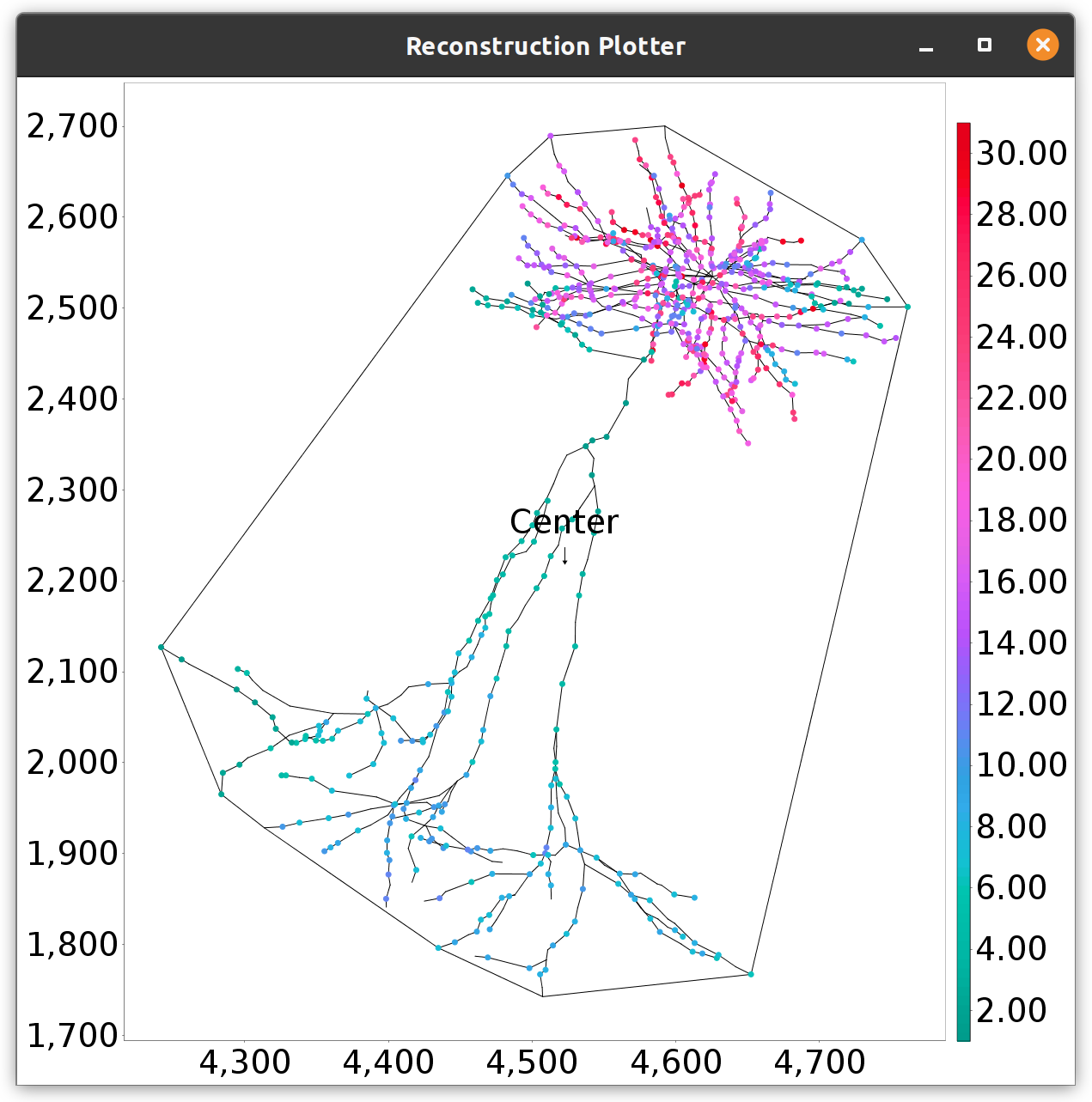 Scripting allows for arbitrary focal points, in this case the centroid of the neuron’s convex hull (Convex Hull as Center template script)
](/media/plugins/snt/shollresultasrois.png) Intersection points and sampling shells can be retrieved as annotation ROIs
Intersection points and sampling shells can be retrieved as annotation ROIs
]](/media/plugins/snt/sholl-rasterized-shells.png) Using Sholl to measure the distribution of image objects (Sholl Rasterize Shells template script) [use case]
Using Sholl to measure the distribution of image objects (Sholl Rasterize Shells template script) [use case]
 can be used to obtain radial maps of fluorescent markers.](/media/plugins/snt/snt-sholl-integrate-density-profiles.png) Not only neurons: Integrated-density profiles can be used to obtain radial maps of fluorescent markers.
Not only neurons: Integrated-density profiles can be used to obtain radial maps of fluorescent markers.
Profile Types
Length-based Profiles
Since SNTv5 it is possible to obtain length profiles in addition to the traditional No. of intersections counts. The two strategies are usually (highly) correlated but not identical: Intersection counts summarize how often the arbor crosses each sampling shell (frequency of crossings). Length summarizes how much cable lies within each shell.
For direct parsing of images, groups of foreground pixels are first identified along each sampling shell:
- Groups are defined as 8‑connected components in 2D and 26‑connected in 3D
- The No. of Intersections at a shell is the number of identified groups
- The Intersected length at a shell is the sum of path lengths of all groups within that shell. Note that lengths can be affected by the apparent thickness of processes. Consider skeletonizing before analysis to reduce thickness bias
For traced morphologies, each segment (straight line between consecutive nodes) is tested against each sampling shell:
- If a segment intersects a shell, the segment is clipped to the shell and its arc length inside the shell is accumulated
- Intersections at a shell correspond to the number of connected arbor components that cross the shell (based on the tracing graph topology, not pixel connectivity)
- Length at a shell corresponds to the sum of Euclidean lengths of all clipped segment pieces inside that shell. Note that node radii are not considered for length calculations
NB:
- Conceptually, length requires a non‑zero radius step size. If you select continuous sampling (step size = 0), the program will internally fallback to a minimum separation: Either the geometric mean of voxel dimension when parsing images, or the median inter-node distance of the structure when parsing reconstructions
- Reported lengths are in calibrated units (e.g., µm)
Intensity-based Profiles
When parsing images directly it is possible to obtain integrated density plots. In this case rather than reporting on No. of intersections or intersected lengths, these profiles report on normalized integrated density. Normalized integrated density is the sum of all voxel intensities along the sampling shell normalized to the perimeter/surface of the shell. These type of profiles can also include cumulative distributions plots and are useful to quantify the distribution of organelles and other structures in cells (including non-neuronal cell types), e.g., as in:
- Distribution of FISH spots within nuclei: doi:10.1371/journal.pgen.1010451
- Distribution of mitochondria: doi:10.1016/j.celrep.2016.09.004
Volume-based Profiles
When parsing tracings, it is possible to profile intersected arbor volume. This is achieved by clipping each traced segment to the sampling shell and summing the volumes of the resulting truncated-cone (frustum) pieces.
Direct Analysis of Images
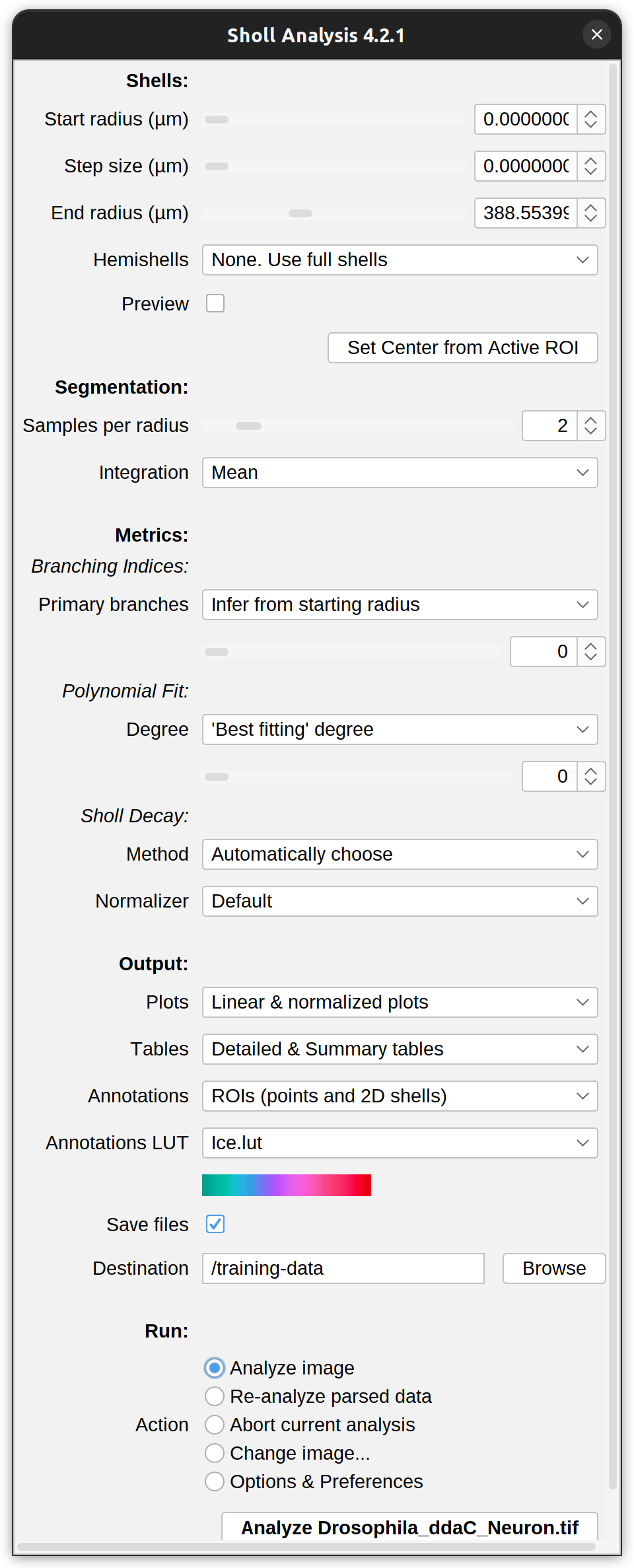
In this mode (bitmap analysis), the plugin requires a binary image or a segmented grayscale image (2D or 3D) containing a single neuron.
- Segment the neuronal arbor using Image › Adjust › Threshold… (shortcut: ⇧ Shift + T). When using multichannel images, you will have to set the display mode to Grayscale using Image › Color › Channels Tool… (⇧ Shift + Z), because images displayed as Composites cannot be thresholded.
- Visually inspect the two thresholded phases in the image to ensure the arbor is being parsed and not background.
- Define the center of analysis using a valid startup ROI.
- Run Analysis › Sholl › Sholl Analysis…, adjusting the default Parameters in the dialog prompt.
- Problems? Read the FAQs.
Startup ROI
The center of analysis can be specified using one of three possibilities:
-
Straight line: A Straight line from the focus of the arbor to its most distal point using the Straight Line Tool. The advantages of using line selections are twofold: 1) Center of analysis and Ending radius are automatically set, and 2) Horizontal/vertical lines (created by holding ⇧ Shift while using the Straight Line Selection Tool) can be used to restrict analysis to sub-regions of the image.
-
Single point: A single point marking the focus of the arbor using the Point Selection Tool. With single point selections, only the center of analysis is defined. Thus, this option is suitable for batch processing of images with different dimensions with undefined Ending radius.
-
Multipoint selection: A Multi-point selection (multipoint counter) in which the first point marks the center of analysis while the remaining points mark (count) the number of primary branches required for the calculation of ramification indices). Suitable for cases in which inference from starting radius is not effective.

Three types of ROIs expected by the plugin when analyzing images directly. Left: Line defining center of analysis (focal point), hemisphere restriction and ending radius. Middle: Single point defining center of analysis. Right: Multi-point selection in which the first point defines the focal point while the remaining points (2 to 5) serve as counters for primary neurites.
Cf. Segmentation
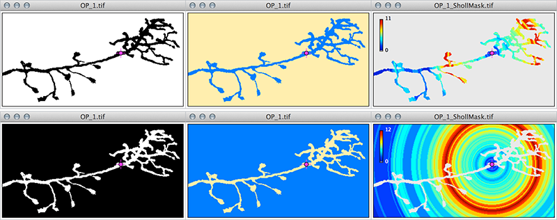
It is important to visually confirm which phase of the segmented image will be sampled, specially when using black and white (binary) lookup tables. To do so, you can select the Red lookup table in the Threshold widget (Image › Adjust › Threshold… ⇧ Shift + T) to highlight foreground from background pixels to verify that you are measuring neuronal processes and not the interstitial spaces between them. Here is an example using an axonal arbor from the Drosophila olfactory neuron demo dataset:
|
Segmented image |
|
|
Note the reversal of output and how the intersections mask no longer decorates the axonal processes but the interstitial spaces between them. The consequences of the phase inversion are twofold: 1) the program oversamples (cf. hue ramps on upper left of Intersections mask) and 2) the program detects artifacts induced by the edges of the image (cf. top-right and bottom-right corners of mask where intersections are sampled in the absence of real axons at those locations). Also, note that the initial black and white image would look the same under an inverted lookup table (Image › Lookup Tables › Invert LUT). |
With binary images, Sholl Analysis treats zero intensities as the background, independently of the image lookup table or the state of the Black background option in Process › Binary › Options…. As with any other ImageJ routine , confusing background with foreground pixels will lead to aberrant results, including: 1) overestimation of branches and 2) artifacts at distances intersecting the boundaries of the image canvas.
Analysis of Traced Cells
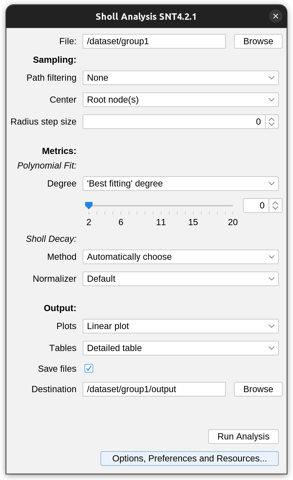
In this mode the plugin analyzes reconstructed arbors (traced in SNT or elsewhere), which is particularly relevant for stainings that do not allow single-cell resolution or proper segmentation. There are several entry points to this analysis, namely:
-
SNT’s main interface: Offers more options for defining the center of analysis, restrictions to tagged branches, etc., but is not amenable to batch processing.
-
Sholl Analysis (Tracings) commands accessed through the Plugins › Neuroanatomy › Neuroanatomy Shortcut Window (SNT icon in the ImageJ toolbar): for cases in which viewing traces is not necessary, or when batch processing is needed
To analyze cells without having to initialize SNT’s tracing interface, run Sholl Analysis (Tracings)… and specify:
-
File The tracing file (swc, .ndf, .json, or .traces extension) to be parsed
-
Path filtering Whether the analysis should be restricted to particular paths, e.g., those tagged as (axon, dendrite, soma, etc.). Note that if your tracings are not tagged you can do so in SNT
- Center The center of analysis, defined by:
- Root nodes These correspond to the starting nodes of primary (root) paths. If multiple primary paths exist, center becomes the centroid (mid-point) of their starting nodes
- Soma node(s) These correspond to nodes tagged as “soma”. If Ignore connectivity is chosen, the centroid of all soma-tagged nodes is used, even if such nodes are not at the root of the structure. If Primary paths only is chosen only root nodes tagged as “soma” are considered
-
Metrics & Output These are described in Curve fitting, Choice of Methods, and Output options.
-
Advanced Options These are included in the Options, Preferences and Resources dialog, and include:
-
Skip somatic segments If primary paths start ‘far-away’ from the soma, this options allows segments between the soma and neurite be ignored. Note that this option is only considered when the arbor being analyzed is rooted on a single-node tagged as ‘Soma’
-
Include zero counts Whether entries associated with 0 intersections should be included in detailed tables, plots, etc.
-
Analysis of Existing Profiles
This option allows curve fitting to be applied to previously sampled profiles and is achieved via scripting. It requires only a tab or comma delimited text file (.csv, .txt) listing a sampled Sholl profile. Have a look at the Sholl Extensive Stats Demo template script for more details.
Parameters
Some parameters are specific to the type of data used as input whether a segmented image or a reconstruction (tracing). When analyzing images, input values take into account the scale information of the image (which can be set using the Analyze › Set Scale… or Image › Properties… (⇧ Shift + P), the type of image (2D or 3D), and its active ROI.
For clarity, settings pertaining to direct parsing of images are tagged with , those pertaining to reconstructions (tracings) with .
Shells
Profile type
Whether the profile should report traditional No. of intersections counts or intersected lengths
Start radius
The radius of the smallest sampling circle/sphere, i.e., the first distance to be sampled.
Step size
The sampling interval between radii of consecutive sampling circles/spheres. This value may be set to zero for continuous (1-voxel increment) measurements. For stacks with anisotropic voxel size, setting Radius step size to zero, sets the step length to the dimension of the matching isotropic voxel, i.e., the geometric mean of voxel dimensions: For 3D images, the cube root of the product of the voxel dimensions; For 2D images: the square root of the product of the pixel dimensions.
End radius
The radius of the largest (last) sampling circle/sphere. It is automatically calculated if a line ROI is used. Note that the specified distance may not be actually sampled, if Radius step size is not a divisor of Ending radius-Starting radius. In this case, the program will choose the largest possible distance smaller than the specified value. You can clear Ending radius or set it to NaN (“Not a Number”) to sample the entire image. This is particularly useful when batch processing images with different dimensions.
Hemishells
This option can be used to limit the analysis to sub-compartments of the arbor. This option instructs the algorithm to measure intersections at sites equidistant from the center that have y-coordinates above/below the drawn line or x-coordinates to the left/right of the center.
Preview
Previews sampling shells on the image being analyzed. Note that with 3D images, the previewed 2D circumferences do not reflect the actual 3D spheres used by the algorithm.
Set center from Active ROI
Updates the center position by reading the centroid of the active ROI.
Noise Reduction
Samples per radius (2D images only)
Defines the number of measurements to be performed at each sampling circumference. These measurements are then combined into a single value according to the chosen integration method. This strategy, a break from previous approaches, increases the accuracy of non-continuous profiles by diluting out the effect of processes extending tangent to the sampling circumference.
Visually, this option can be imagined as the “thickness” of the sampling circumference: e.g., for a radius of 100 pixels and a value of 3 Samples per radius, the final number of intersections would integrate the measurements sampled at distances 99, 100 and 101. Note that it would not make sense to increase the number of samples beyond the length (in pixels) of Radius step size. For this reason, this option is limited to a draconian (and arbitrary) maximum of 10 samples.
Samples integration (2D images only)
The measure of central tendency used to combine intersection counts when multiple Samples per radius are used. Options are Mean (the default), Median or Mode.
Ignore isolated voxels (3D images only)
Accessed through the Options & Preferences dialog. If checked, single (6-connected) isolated voxels intersecting the surface of sampling spheres are not taken into account, which may allow for smoother profiles on noisy image stacks. However, it should be noted that connectivity in the stack volume may not reflect connectivity on the surface of a digitized sphere. Indeed, in certain contexts, it is possible (though unlikely) to obtain higher intersection counts when this filtering option is active.
Keep in mind that this is just a refinement feature, and you should not expect it to mitigate major artifacts derived from poor segmentation.
No. of parallel threads (3D images only)
Accessed through the Options & Preferences dialog. Sets the max. no. of parallel threads to be used when parsing 3D stacks. Note that this options also sets the no. of threads used by ImageJ and SNT for other multithreaded tasks. Set it to 0 to use all of the available processors on your computer.
Number of primary branches
The number of primary branches (i.e., those originating directly from cell soma when the center of analysis is the perikaryon) to be used in the calculation of Schoenen ramification indices. This option is only relevant when computing branching indices. Set it to zero to disable calculations of ramification indices. Choices include:
- Infer from starting radius If checked, the Number of Primary branches is inferred from the count of intersections at Starting radius.
- Infer from multipoint ROI Uses multipoint counts if a multipoint ROI is detected at startup.
Polynomial fit
Specifies the degree of the polynomial to be fitted to the Linear profile3. While the polynomial of best approximation, or “best fit”, should be empirically determined for each analyzed cell type, it is possible to ask the plugin to predict the order of the fitting polynomial (or at least try) using the choice Best fitting degree. In this case, the plugin will loop through all the available choices of polynomials, perform each fit in the background and choose the one with the highest coefficient of determination.
Detailed control over polynomial fitting is controlled by the options in the Options & Preferences prompt, namely:
- Min. Degree The lowest order to be considered when calculating the ‘best-fit’ polynomial
- Max. Degree The highest order to be considered when calculating the ‘best-fit’ polynomial (degrees above 40 may not be supported)
- R-squared cutoff The coefficient of determination (R2) cutoff used to discard ‘inappropriate fits’. Only fits associated with a R^2 greater than this value will be considered
- K-S validation Whether a fit should be discarded if two-sample Kolmogorov-Smirnov testing rejects the null hypothesis that fitted and profiled values are samples drawn from the same probability distribution (p<0.05)
Normalization
Options for computing metrics based on normalized (Semi-log or Log-log profiles), including Sholl decay.
-
Method Specifies the type of method. Select Automatically choose when you cannot predict which type of normalized profile best describes the dataset. If chosen, the plugin will use the Determination ratio to determine which of Semi-log or Log-log methods is more appropriate.
-
Normalizer The property of the sampling shell to be used in the normalization of Linear-norm, Semi-log, and Log-log profiles. Default is area (2D images)/volume (3D images). It is described below.
Output Options
Defines which kind of annotations should be output, including:
-
Plots The type of plot(s) to be output. In addition to the Linear and Normalized profiles, it is also possible to obtain polar plots, as well as cumulative distribution plots for intensity-based profiles.
-
Tables Defines which kind of tables should be output, including Detailed and Summary tables.
-
Annotations Defines which kind of annotations should be output, including:
-
LUT The Lookup Table (LUT) used for annotations.
-
ROIs Allows for two sets of ROIS to be added to the image overlay: 1) concentric shells matching sampled distances (circular ROIs or composite ROIs when using hemicircles); and 2) Multipoint ROIs at intersection sites between shells and clusters of foreground pixels. Note that WYSIWYG versions (RGB images) of these masks can be obtained using by pressing ⇧ Shift + F (Image › Overlay › Flatten) or by running Analyze › Tools › Calibration Bar….
NB:
- ROIs are not created when outputting integrated density
- Versions prior to SNTv5 placed intersection points at edges of detected clusters of foreground pixels, not their centroid
-
Mask A 16/32–bit maximum intensity projection of the analyzed image is generated in which the measured arbor is painted according to its Sholl profile. The type of data (Raw, i.e., sampled or Fitted) is displayed in the image subtitle
-
-
Save files If checked, outputs are saved to the specified directory. Files are named after the image filename .
-
Show fitting details - Choose this option to have all the parameters of the simplex fitting printed to the Log window. The coefficient of determination (R2, a measure of goodness of fit) is always stored in the Sholl Results table even when this option is not selected
Sholl Plots
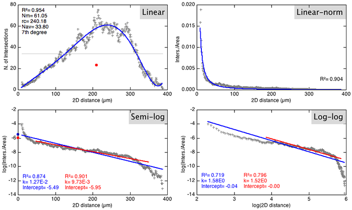
Linear, Linear-norm, Semi-log and Log-log profiles for the ddaC demo dataset. Most of the retrieved metrics are automatically highlighted by the plugin. Linear profile: Mean value (horizontal grid line) and Centroid (colored mark). Logarithmic profiles: The Sholl regression coefficient (also known as Sholl decay) can be retrieved by linear regression using either the full range of data (blue line) or data within percentiles 10–90 (red line). For this particular cell type, the Semi-log method is more informative when compared to the Log-log method. See Angular Sholl for other types of plots.
|
Method |
Fit |
Description |
|
|---|---|---|---|
|
(1) |
Linear |
N = a + br + cr2 + dr3 + er4 + fr5 + ... + xrn |
|
|
(2) |
Linear-norm |
N/S = a rb |
|
|
(3) |
Semi-log |
log(N/S) = -k r + m |
|
|
(4) |
Log-log |
log(N/S) = -k × log(r) + m |
|
|
(5) |
Angular (Polar) |
von Mises (unimodal distributions only) |
|
N For 2D images, the Number of clusters of pixels (8–connected) intersecting the circumference of radius r
For 3D images, the Number of clusters of voxels (26-connected) intersecting the surface of the sphere of radius r
r Distance from center of analysis (radius of Sholl circle/sphere)
log Natural logarithm, the logarithm to the base e
S The property of the sampling shell to be used in the normalization of Linear-norm, Semi-log, and Log-log profiles. For 2D images, the Perimeter of the sampling circumference (2πr) or the Area of the corresponding circle (πr2) For 3D images, the Surface of the sampling sphere (4πr2) or its respective Volume (4/3πr3) Annulus/Spherical shell normalization is also available when performing non-continuous sampling. In this case, the normalization is performed against the area/volume between circumferences/spheres at r ± Radius step size/2
Angular Sholl
Angular Sholl (radius × angle, also called Polar Sholl) produces polar heatmaps to reveal directional biases in Sholl Profiles and how such biases change with distance. Angular Sholl distributes the location of Sholl intersection (i.e., “Sholl Points”) over angular sectors. Summing the No. of intersections (or intersected length) across each radius produces an angular distribution used to compute angle-based metrics.
In simplistic terms, the algorithms in Angular Sholl that detected preferred orientations work as follows:
-
“compass histogram”: Imagine the space around the neuron divided into equal slices like a pizza (e.g., every 10°). For each slice the program adds up how much arbor points each way—either the number of crossings (“intersections”) or the amount of intersected cable (“length”)
-
Smoothing: Each slice is averaged with its two neighbors to reduce jitter from noise
-
Standout slices (“peaks”) are identified: The program measures how much “taller” a slice is relative to its immediate neighbors using a local prominence (difference from the average of the two neighbors). Only taller slices with a strong prominence are considered real peaks
-
Curve fitting: If only one peak is identified, the distribution angles is fitted to a von Mises distribution. As detailed in Root Angle Analysis, this a circular analogue of the normal distribution that models angles/directions
-
After this process is concluded, a list of directional “peaks” are obtained: each has an angle (in degrees) and a strength (the height of that slice)
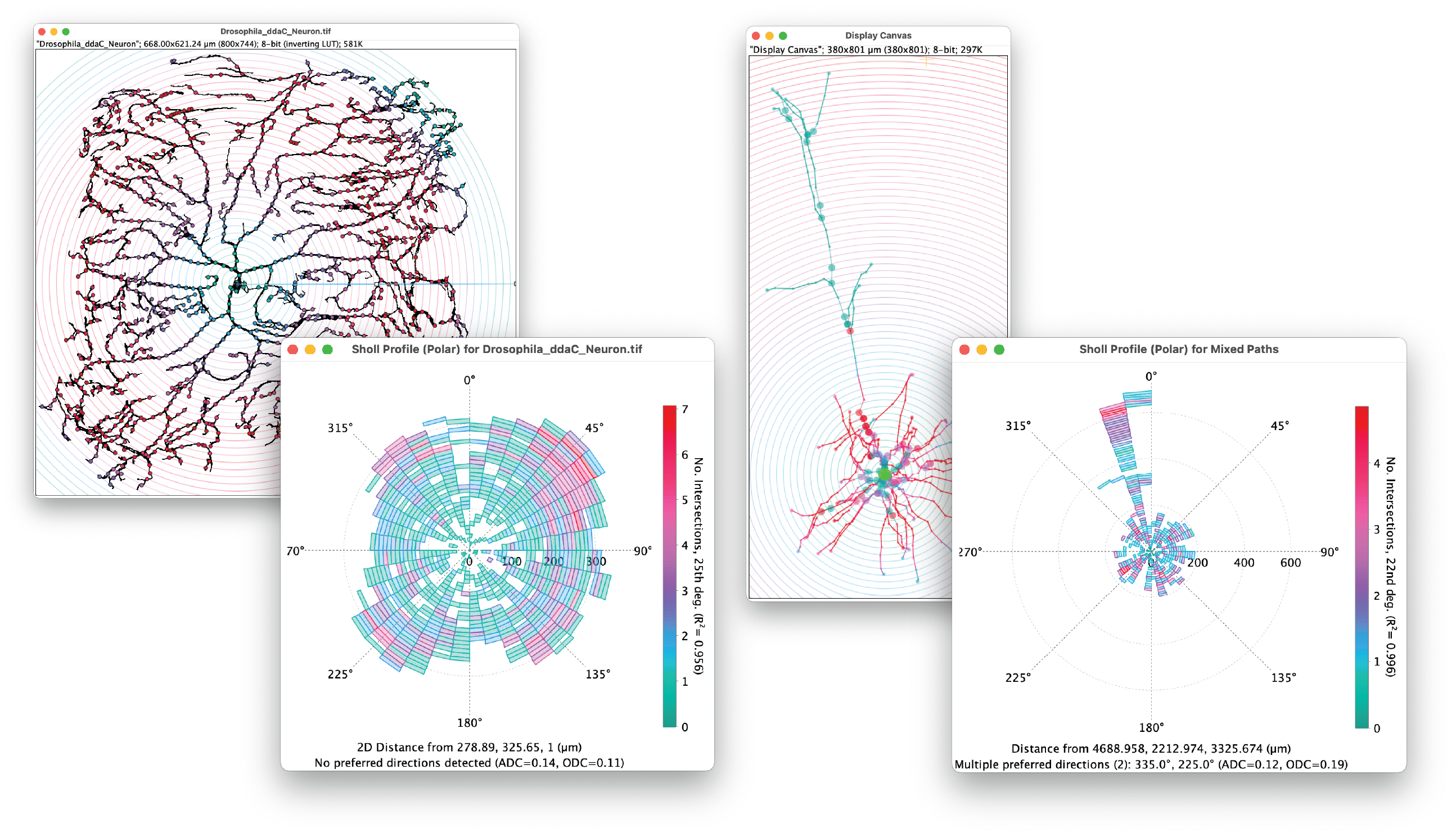 Examples of angular (polar) profiles. Left: Space filling dendrites of the ddaC demo dataset featuring a homogeneous angle distribution. Right: Pyramidal neuron (MouseLight dendrites demo dataset). Basal dendrites are associated with an homogenous angle distribution, but apical dendrites feature a strong directional bias. In both causes, a bin width of 10° was used. This type of data can be obtained for length-based profiles and fitted data.
Metrics
Morphometric descriptors and other properties of the arbor are printed to the measurements table. Output is customizable using the detailed metrics checkbox in the “Further Options” dialog in the analysis prompt.
Metrics based on sampled data
-
Branching Index (BI) An index that summarizes neurite arborization as defined by Garcia-Segura & Perez-Marquez4. Note that this index is broadly affected by radius step size. Comparison of this metric across cells sampled differently will be nonsensical, as demonstrated here. Step size should always be included (e.g., BI10μm=20) when reporting this metric.
-
Centroid radius The abscissa of the centroid (i.e., the geometric center or barycenter) of the linear profile. It is highlighted on the N vs Distance plot.
-
Centroid value The ordinate of the centroid (i.e., the geometric center or barycenter) of the linear profile. It is highlighted on the N vs Distance plot.
-
Enclosing radius The last (thus, the widest) of Intersecting radii to be associated with the number of intersections specified by Enclosing radius cutoff. For a cutoff of 1 (the default) Enclosing radius is the widest of Intersecting radii. It reflects the Feret length of the arbor.
-
Kurtosis The kurtosis of the sampled data, which quantifies whether the shape of the distribution matches that of a Gaussian distribution, assuming that a Gaussian distribution has a kurtosis of 0. A distribution more peaked than a Gaussian has a positive kurtosis while a negative value indicates a flatter distribution. See also Kurtosis (fitted data)
-
Highest count of intersections (Max inters.) The maximum value of sampled intersections, i.e., the maximum in a linear [N vs Distance] profile, reflecting the highest number of processes/branches in the arbor. See also Critical value.
-
Intersecting radii The number of sampling radii intersecting the arbor at least once.
-
Mean of intersections (Mean inters.) Sum inters. divided by Intersecting radii. See also Mean value, FAQ
-
Median of intersections (Median Inters.) The median value of sampled intersections.
-
Radius of highest count of intersections (Max inters. radius) The distance at which the Highest count of intersections occurred, reflecting sites of highest branch density. Note that if the same maximum occurs multiple times, only the first distance is considered. See also Critical radius
-
Schoenen Ramification index (Ramification index (sampled)) A measure of ramification5: the ratio between Max inters. and the number of primary branches. It is only calculated when primary branches is valid and not zero. See also Ramification index (fit)
-
Skewness The skewness of the sampled data, an indication of how symmetrical the distribution is around its mean. Positive values indicate an asymmetrical distribution with a longer tail to the right. Negative values indicate data with a longer tail to the left. A popular rule of thumb considers that if the skewness is greater than 1.0 (or less than -1.0), the distribution may be considered far from symmetrical. See also Skewness (fitted data)
-
Sum of intersections (Sum inters.) The sum of all intersections.
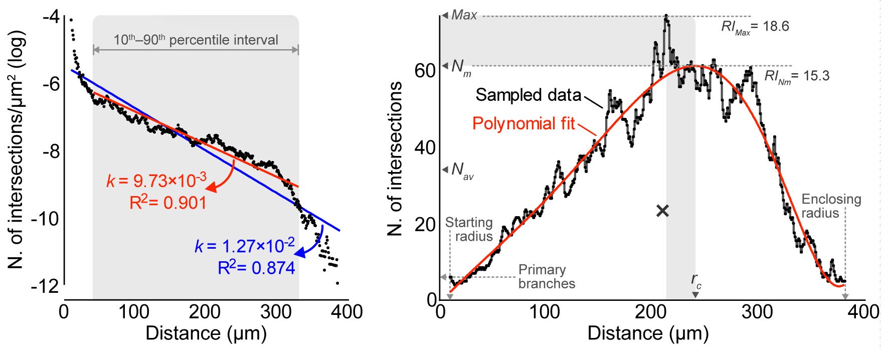 Overview of Sholl metrics) based on curve fitting including the Sholl regression coefficient (k), Critical value (Nm), Critical radius (rc) and Mean value (Nav). Differences between sampled and fitted maxima are shaded in gray. The centroid of the sampled profile is marked (×). Schoenen ramification index (RI) is the ratio between number of branches at the maximum and the number of primary branches, using either sampled data or the fitted Nm. (Ferreira T, et al., 2014, supplementary booklet)
Metrics based on fitted data
-
Branching Index (BI fitted) the branching index obtained from the fitted profile.
-
Critical radius The distance at which Critical value occurs. By default, it is calculated with a precision of 1/1000 of Radius step size. Abbreviation: rc. See also Max inters. radius
-
Critical value The local maximum of the polynomial fit, i.e, N at Critical radius in (1). Abbreviation: Nm. See also Max inters.
Nomenclature: Previous authors have used different terms to describe the largest value taken by the Sholl profile, including Dendrite maximum. Since the Sholl technique is not restricted to dendritic arbors and can be applied to any tree-like structure such as axonal arbors, mammary ducts or blood vessels (cf. List of citations), Here we adopt the term Critical radius, renaming Dendrite maximum (Nm) to Critical value.
-
Determination ratio The ratio of the coefficient of determination for the semi-log method and that for the log–log method6. If the semi-log method is better relatively to the log–log method, the Determination ratio becomes larger than 1. It is the parameter used by the plugin to silently predict the normalization method that is the most informative. The prediction can be monitored by selecting Debug mode in Options and Preferences.
-
Kurtosis (Kurtosis (fit)) The kurtosis of the fitted polynomial distribution between Starting radius and Ending radius.
-
Mean value The mean value3 of the fitted polynomial function (1), representing the average of intersections over the whole area occupied by the arbor. Abbreviation Nav. On the Sholl plot, it is highlighted as the height of the rectangle that has the width of Enclosing radius − First intersecting radius and the same area of the area under the fitted curve on that discrete interval. It is analogous to Mean inters., the arithmetic mean of sampled intersections throughout the arbor (cf. Metrics based on sampled data). By default, (see Advanced Usage), it is calculated with a precision of 1/1000 of Radius step size.
-
Polynomial R2 (Polyn. R^2) The coefficient of determination of the polynomial fit described in (1).
-
Regression intercept The y-coordinate m described in (3) and (4).
-
Regression R2 (Regression R^2) The coefficient of determination of the linear regression described in (3) and (4).
-
Schoenen Ramification index (Ramification index (fit)) Schoenen Ramification index retrieved from fitted profile: The ratio between Critical value and Number of primary branches. See also Ramification index (sampled)
-
Sholl regression coefficient (Regression coefficient) The slope (multiplied by -1) of the linear regression described in (3) and (4), i.e., k, a measure of the rate of decay of the number of branches with distance from the center of analysis. Higher k values reflect larger changes in the function log(N/S). To optimize the fit, the plugin retrieves a second linear regression centered around the median distance, excluding distances at the edges of the profile. Details of this second fit are also registered on the Sholl table under dedicated columns, e.g., Sholl regression coefficient [P10-P90], when data within the 10th–90th percentile is used.
-
Skewness (Skewness (fit)) The skewness of the fitted polynomial distribution between Starting radius and Ending radius.
Metrics based on Angular Sholl
-
Angle distribution coherence (ADC) The evenness of the angular distribution of Sholl data. Unitless, ranging from [0, 1], with higher values indicating Sholl data is concentrated around a preferred direction; 0 indicates a uniform distribution across all directions.
-
Preferred directions (PD) The direction around which Sholl data is the most concentrated when Angle distribution coherence is high. Range: [0°,360°[. Examples: A space filling neuron is not expected to be associated with a prominent direction (low ADC value). On the other hand, a cell may have more than one preferred direction (e.g., data from dendrites of a pyramidal neuron), as exemplified above.
-
Orientation distribution coherence (ODC) This is a variant of Angle distribution coherence that considers orientation as opposed to direction. ODC can be useful to discriminate morphologies that are symmetric across 180° (e.g., a neuronal arbor with two opposite tufts) for which ADC can be near 0
-
Preferred orientations The orientation around which Sholl data is the most concentrated when Orientation distribution coherence is high. Range: [0°,180°[
Similarly to all other Sholl-related profiles, both intersection counts and intersecting lengths can be used, as well as data from polynomial fits. By default, polar heatmaps use an angular bin width of 10°. This sensitivity can be adjusted in the “Further Options” dialog in the analysis prompt.
Complementary Tools
SNT provides several scripts and commands that facilitate all types of Sholl-related analyses. You’ll find them through the Plugins › Neuroanatomy › Neuroanatomy Shortcut Window (SNT icon in the ImageJ toolbar), as well as in Script Editor’s Templates › Neuroanatomy menu.
For more information on image processing routines have a look at tutorials, segmentation and the ImageJ User Guide .
Pre-processing
This section discusses some aspects that should be taken into account when segmenting neuronal arbors to be processed by Sholl Analysis. Since image segmentation (i.e., the partitioning of images into analyzable parts) is vulnerable to noise and background fluorescence, it is not possible to generalize universal routines that efficiently binarize grayscale images. This means that any procedure that tries to appropriately describe the original fluorescence image with a binary mask must be tailored to the characteristics of individual datasets.
Noise
Noise can be mitigated through the usage of processing filters. Especially useful are edge-preserving filters:
- Tubeness and Frangi, see SNT’s Secondary Layer Wizard
- Rolling Ball or “Top hat” filters, e.g., Process › Subtract Background…
- Median Filtering (2D/3D), e.g., Process › Filters, Plugins › 3D
- Anisotropic Diffusion, Plugins › Process › Anisotropic Diffusion 2D
- Sobel Edge Detection, e.g., Process › Find Edges
- Shen-Castan Edge Detector (BAR plugin), BAR › Segmentation
- Frequency filters, e.g., Process › FFT › Bandpass Filter…
Uneven Illumination
Uneven illumination problems, typically associated with wide field microscopy, do occur in confocal microscopy when signal from deep layers of the tissue is not captured as bright as with superficial layers. This signal attenuation along the Z-axis will generate a shaded gradient across the stack that histogram-based segmentation will need to take into account. While these problems are better tackled during acquisition (e.g., using laser ramping), it is possible to mitigate this effect using histogram-normalization techniques. E.g.:
- Tubeness and Frangi, see SNT’s Secondary Layer Wizard
- Bleach Correction, Image › Adjust
- Attenuation correction
Segmentation
It is possible to adopt more sophisticated segmentation algorithms when global thresholding methods do not yield satisfactory results. Examples:
- Machine learning algorithms (semantic segmentation)
- Local Threshold, Image › Adjust
- Robust Automatic Threshold Selection, Plugins › Segmentation
- Level Sets, Plugins › Segmentation
- Morphological Segmentation, Plugins › Segmentation
- Squassh, split-Bregman Image Segmentation (Segmentation and Quantification of Sub-cellular Shapes, MOSAIC ToolSuite, Plugins › Mosaic › Segmentation
- MorphoLibJ
- BAR scripts for manual curation of thresholded images, BAR › Segmentation
Batch Processing
SNTv5 reinstated macro-recordable commands. So the easiest/quickest way to automate analysis requires only a few steps:
- Open ImageJ’s macro recorder: Plugins › Macro › Record…
- From the Neuroanatomy Shortcuts Window, choose the relevant prompt from the Macro Recordable section of Sholl Analysis ›
- Set the options as usual
- Copy the recorded string into your macro/script. Beware that the recorded expression is quite large. Make sure to avoid copy/paste errors. It should look something like:
// NB: have a look at the example scripts in Templates>Neuroanatomy> for more robust ways to automate Sholl. E.g., Sholl_Extract_Profile_From_Image_Demo.py exemplifies how to parse an image programmatically using API calls
run("Sholl Analysis (From Image)...", "datamodechoice=Intersections startradius=0.0 stepsize=10.0 endradius=400.0 hemishellchoice=[None. Use full shells] previewshells=false nspans=1 nspansintchoice=N/A primarybrancheschoice=[Infer from starting radius] primarybranches=0 polynomialchoice=['Best fitting' degree] polynomialdegree=0 normalizationmethoddescription=[Automatically choose] normalizerdescription=Default plotoutputdescription=[Linear, normalized, and polar plots] tableoutputdescription=[Detailed & Summary tables] annotationsdescription=[ROIs (points and 2D shells)] lutchoice=Ice.lut save=true savedir=/Users/ferreirat analysisaction=[Analyze image]");
For more comprehensive functionality, the Script Editor’s Templates › Neuroanatomy menu lists demo scripts that perform batch operations. For sake of completeness, here is a small tutorial on how to write a macro from the ground up:
Tutorial: Batch Analysis of Images using IJ Macro Language
Any macro must set a center, or allow the Sholl Analysis plugin to access a ROI marking it. One could instruct ImageJ to read the coordinates of pre-existing ROIs from a text file, store a list of line selections in the ROI Manager, or write a morphology-based routine that detects the center of the arbor. However, marking the center of analysis is probably something that you will want to do manually. Here is a workflow:
- Place all the .tif images to be processed in a single folder.
- Select the Point Selection Tool in the main ImageJ window. With 3D images, make sure Set stack positions is active in the Image › Overlay › Overlay Options… prompt.
- Open the first image and press ⇧ Shift + T to activate the Threshold widget (Image › Adjust › Threshold…).
- Adjust threshold levels. Press the Apply button of the Threshold widget to create a binary image.
- Select the z-slice containing the center of analysis. Click over the center with the Point Selection Tool and press B (shortcut for Image › Overlay › Add Selection…). This will add the point ROI to the image overlay. Save the image as .TIFF by pressing S (File › Save As… › Tiff…).
- Repeat the last 2 steps until all images are marked, using ⇧ Shift + O (shortcut for File › Open Next) to iterate through all the images.
When working with ROIs, it is critical that you work with .tif files because only this format keeps track of image overlays. IJ’s Process › Batch › Convert… command allows bulk conversion between image formats.
Now that all the images are marked, we could use the Macro Recorder (Plugins › Macros › Record…) and run Sholl Analysis on one of the images to find out how to call the plugin with suitable parameters. In this tutorial, we will use the ImageJ macro language. The single line of code that appears in the recorder window will look something like this:
// Recording Sholl Analysis version 3.4.3
run("Sholl Analysis (From Image)...", "datamodechoice=Intersections starting=10 ending=400 radius_step=0 infer fit linear polynomial=[8th degree] semi-log normalizer=Volume create save do");
As you may have noticed, ImageJ plugins are controlled by a single lowercase sentence in which arguments are separated by a space. Input fields and choice lists appear as keyword=value pairs, active checkboxes by a single keyword. Options that are not needed can be omitted. This makes it easier to edit code blocks:
start = 10;  // variable that controls starting radius
end   = 200; // variable that controls ending radius
step  = 2;   // variable that controls step size

// Run the plugin
run("Sholl Analysis (From Image)...", "starting="+ start +" ending="+ end +" radius_step="+ step +" infer linear save do");
Now we just need to assemble a working macro to be pasted in the Process › Batch › Macro… prompt:
// Get the number of ROIs of the image overlay
nROIs = Overlay.size;
// We cannot proceed if no ROI is available (safety check)
if (nROIs==0)
    exit("No ROI was found. Cannot proceed.");
// Select the last ROI of the overlay. Because we have activated the "Set stack positions" option,
// this will automatically activate the Z-slice in which the ROI was created (3D images)
Overlay.activateSelection(nROIs-1);
// We now call the plugin as detailed by the Macro Recorder. We'll set 'Ending radius' to a non-numeric
// value (NaN, "Not a Value") to make sure the maximum length for each individual image is used
run("Sholl Analysis (From Image)...", "datamodechoice=Intersections starting=10 ending=NaN radius_step=0 infer fit linear polynomial=[8th degree] semi-log normalizer=Volume create save do");
Of course you can also automate any preceding steps. However, do not forget to ensure that the center of analysis will be available when the plugin is called:
// Impose spatial calibration
run("Properties...", "unit=um pixel_width=1.5 pixel_height=1.5 voxel_depth=3.0");
// Subtract background
run("Subtract Background...", "rolling=50 sliding stack");
// Apply a favorite threshold
setAutoThreshold("Huang dark stack");
// >>>> Make sure the initial point selection remains available <<<<
Overlay.activateSelection( Overlay.size - 1 );
// Run the plugin
run("Sholl Analysis (From Image)...", "datamodechoice=Intersections starting=10 ending=NaN radius_step=0 infer fit linear polynomial=[8th degree] semi-log normalizer=Volume create save do");
That’s it. Use the Macro Recorder to generate the customizations you will need before parsing the entire folder of images with Process › Batch › Macro…
Complex Scripts
More complex scripts will take advantage of SNT’s API. Here are some of scripts from SNT’s Bundled Templates:
FAQ
For clarity, FAQs pertaining to direct parsing of images are tagged with , those pertaining to reconstructions (tracings) with .
General
-
How do I cite Sholl Analysis?
-
The authoritative references for Sholl Analysis are twofold:
-
Why do I need to threshold the cell?
-
Counting intersections is really a binary procedure: a shell either intercepts a branch or it doesn’t. For this reason the image must be split in two phases: arbor and background.
-
In older versions it was not mandatory to adjust threshold values prior to analysis. Why is it now?
-
Image segmentation has always been required. In its early implementations, the program dealt solely with binary images and used the intensity at the center of the analysis to decide how to segregate objects from background. This approach was very stringent: It assumed that the pixels representing the neuron would have the same (constant!) intensity that was not to be found in the remaining background. As the program became aware of grayscale images, this “feature” had to be removed because a single intensity can no longer be used to infer which parts of the image should be analyzed.
-
My images do not look that great. How can I treat them prior to analysis?
-
Have a look at Pre-processing.
-
My bitmap profiles are different from the ones obtained from tracings of the same cells. Why?
-
The quality of the analysis relies on how the arbor was segmented. If you are working with grayscale images you may need to optimize your segmentation routines. On the other hand, if you already obtained binary images make sure you are interpreting them properly. You should also confirm that Ending radius does not intersect other structures in the image beyond the analyzed arbor. See also The 3D profile looks worse than the 2D profile of the Maximum Intensity Projection of the same cell. Why?
-
My version is not the latest after running Help › Update Fiji… Why?
-
This may happen if you have manually installed/modified core files.. Run the Updater, choose Advanced Mode then View locally modified files under View Options. Locate files from the Neuroanatomy update site. If the Details pane indicates an available update, click on Locally modified under Status/Action and choose Install/Update. The latest release version will be available once you press Apply changes. See Installation FAQs for more details.
-
This documentation is not that useful. How long do I have to wait until it gets improved?
-
Use the Edit this page option on the top of the page and edit its contents at will. Don’t be shy. All changes are undoable!
Analysis
-
The plugin complains about a wrong image type. Why?
-
The plugin does not parse RGB images, but will process any grayscale image (8/16-bit), including multichannel (composite) images. This is intentional: RGB images are inflexible and images of fluorescence-labeled cells are typically non-RGB images. As explained in the ImageJ User Guide, RGB images can be converted using Image › Color › Channels Tool… or Image › Type commands.
-
With 3D and 4D images, how do I set the Z-position of the center?
-
The Z-position (depth) of the center of analysis is the active Z-slice of the stack. With multichannel (composite) images, the active channel also defines the C-position. Both are reported in the Sholl Results table.
-
Why so many parameters?
-
The plugin is designed for the analysis of a wide diversity of arbors and it is not biased to any particular cell type. The only way to ensure this broad applicability is to give users full control over the mathematical techniques used by the plugin to analyze sampled data.
Results
-
How can I save/edit the Sholl Results table?
-
Use Fiji’s File › Export › Table… command or SNT’s File › Save Tables and Analysis Plots… (details), or right-click on the table and choose Save As…
-
What is the Sholl mask?
-
The Sholl mask (see example of CA1 cell) is simply an illustration: a maximum intensity projection of the analyzed cell in which intersection counts are used as pixel intensities. As explained in Output Options, its LUT can be modified, and intensities calibrated using ImageJ default commands. As mentioned, it can also be used to visually inspect for segmentation artifacts.
-
The 3D profile looks worse than the 2D profile of the Maximum Intensity Projection of the same cell. Why?
-
An anisotropic voxel size will have a strong impact on step size. On the other hand, 2D and 3D images can be sampled differently depending on the options chosen. If Image › Properties… (⇧ Shift + P) reports the appropriate spatial calibration, check Noise Reduction parameters. The Analysis › Sholl Bitmap vs Tracing Comparison template script can be used to compare Sholl profiles across different inputs (2D/3D images vs 2D/3D reconstructions).
-
The program terminates without warnings. What am I doing wrong?
-
The program should not terminate without throwing an error message.
Metrics and Curve Fitting
-
Would it be possible to retrieve the Area Under the Curve (linear Sholl plot)?
-
The area under the curve (AUC, the area between the sampled curve and the horizontal axis, i.e., its definite integral) could be estimated using, e.g., the trapezoidal rule. However, because data is always sampled at equally spaced intervals, doing so would be the same as multiplying Mean inters. by the distance between Ending radius and Starting radius. Thus, effectively, AUC is redundant with Mean inters., that is already an integrated measurement of the sampled data. On the other hand, one could retrieve the AUC of the polynomial fit, but such property is already covered by Mean value.
-
The shape of the polynomial changes at the edges of the profile. Why?
-
Inflection points at starting/ending radius are usually associated with a poor fit and/or the fact that all the radii in which no intersections were counted are ignored. The latter is required to calculate the Sholl regression coefficient, as log(0) is undefined.
Batch Processing
-
The code that the Macro Recorder produced does not seem to work. What am I doing wrong?
-
Note that the Neuroanatomy Shortcuts Window lists two types of commands: Interactive and Macro Recordable. The latter should be used for efficient macro recording. Frequent interactions with the interactive dialog prompt(s) (from which the Recorder retrieves user-specified parameters) can “confuse” ImageJ. The solution is to repeat the recording with Macro Recordable commands.
Development
-
I found a bug. How do I report it?
Version History
Release notes are available on the SNT repository. Releases notes up to version 3.7.3 are available on an older repository. In turn, the latter inherited (with permission) the 2D algorithm of an even earlier ImageJ 1.35 plugin by Tom Maddock. Note that throughout 2012 the project was temporarily called Advanced Sholl Analysis.
Publication
Citing manuscripts can be retrieved using Scholar or PubMed, although many more publications seem to be using it. See Global FAQs for details on how to cite SNT.
References
-
Sholl DA. Dendritic organization in the neurons of the visual and motor cortices of the cat. J Anat. 1953 Oct;87(4):387-406. PMID: 13117757 ↩

 and [Angle-based metrics](#metrics-based-on-angular-sholl)](/media/plugins/snt/snt-angular-sholl-ddac.png)