This page was last revised for version 5.0.5.
Please help us to keep these walkthroughs up-to-date by editing this page directly to fill in any documentation gap. Do reach out if you need assistance!
Semi-automated Tracing
You can follow these instructions using File › Load Demo Dataset… and choosing the Drosophila OP neuron (Complete 3D reconstruction) dataset. All the neuronal processes are traced in this dataset, so you may want to delete some of the existing paths beforehand.
These instructions assume that you have read the Manual, including starting up the plugin, enabling Cursor Auto-snapping, and Auto-tracing options. Parts of this section are also documented in a Screencast.
Starting A Path
I. Pick The Starting Point
 You may notice that, by default, the cursor snaps to the brightest pixel in its vicinity. If you prefer to manually control the placement of nodes, feel free to toggle this feature by pressing S. Now, to begin tracing, move through the image stack to find the start point of a path then click there with the left mouse button.
II. Pick A Subsequent Point
 A small circle should appear, highlighting the start of the path. Move through the stack to find a subsequent point further along the same structure to be traced (neuron, blood vessel, etc.), and click there.
If a path between the two points cannot be found immediately, you may see the animated progress of the search. You can scroll through the stack while such a search progresses: If it appears to not be making good progress, it’s probably best to press the “Cancel/Esc” button (shortcut: C/⎋ Esc) and pick a point closer to the start point.
 NB: You can always press Z to undo the last segment
NB:
- Increasing Z in the Cursor Auto-snapping panel allows for automated Z-navigation on signal mouseover
- You can increase the contrast (opacity, size, etc.) of Path nodes in the Path rendering widget of the Options tab
Use ⌃ Ctrl + Mouse Wheel to change the diameter of the path being traced, by adjusting the cursor size to the thickness of the neurite being traced.
III. Confirm The Temporary Segment
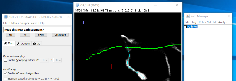
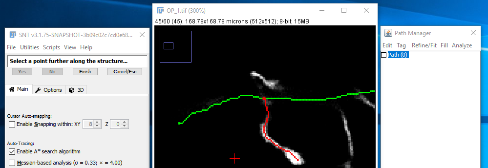
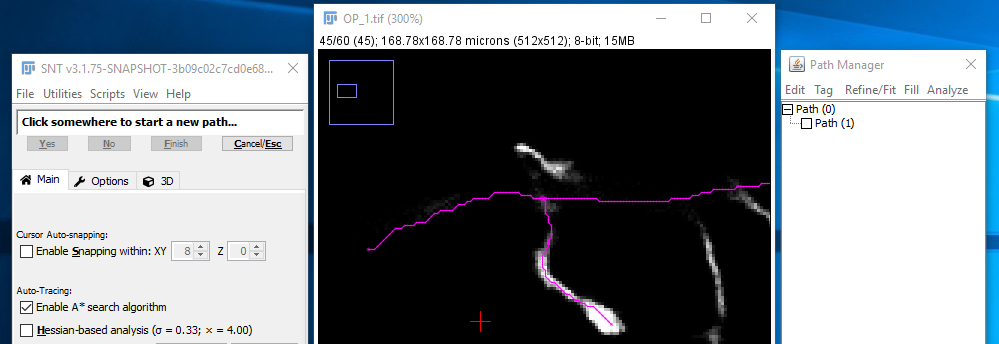
Once the search has reached the target point, the path is shown in cyan (to indicate that this is still a temporary path) and you are asked to confirm (by clicking “Yes” or pressing Y) that this path is following the route through the image that you expect. If it is not, then click “No” N and you’ll go back to the previous step. Assuming you confirmed the path, the confirmed path will appear in red. Now you are essentially back at step II. Normally you will go on to pick further points along the structure. However, if you have finished with that path, click “Finish Path” F and you will go back to step I. If you completed that path it would be shown in magenta.


NB: Once you become familiarized with the software you may want to disable the confirmation of temporary segments in Temporary Paths section of the Options tab.
This will allow you trace faster by finishing a path using Double Click, and using Z to undo any misplaced segment.
Hold O to verify path orientations. Hold H to temporarily hide all annotations.
Branching: Start A Path On An Existing Path
I. Select The Path To Branch Off
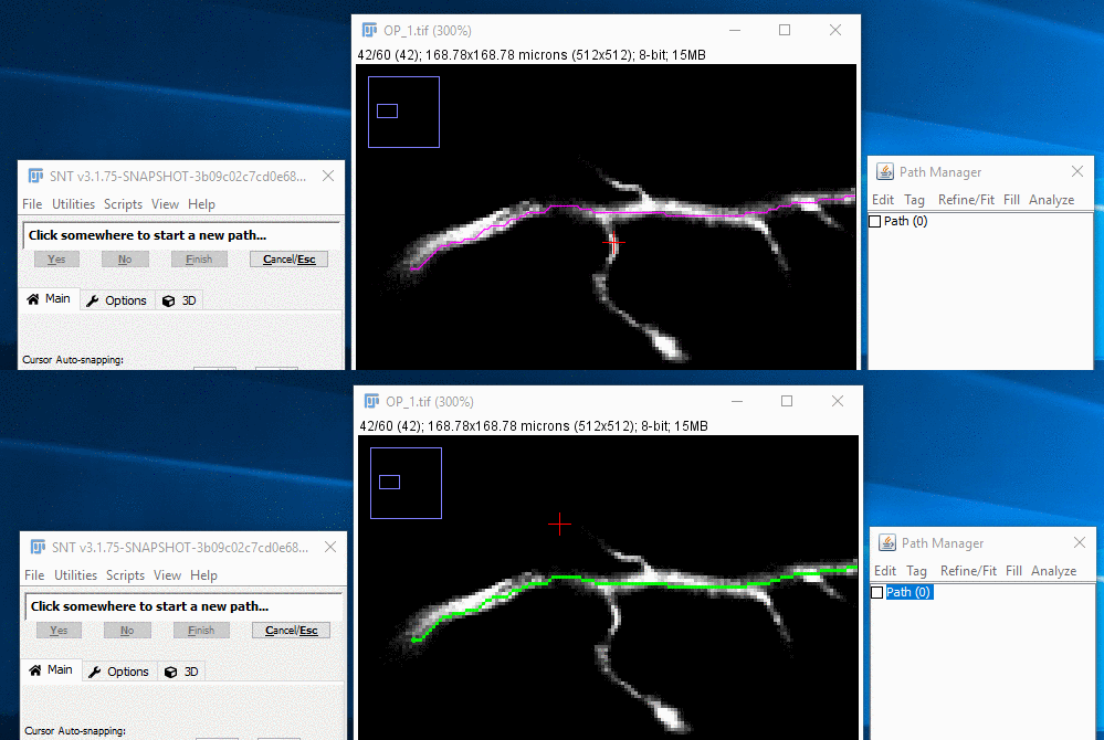 To select the path you want to branch off from, you can either select it in the Path Manager, or press G while the mouse pointer is near the path. When the path is first selected, it will be shown in the default green color. Note that you can also right-click on the image and choose Select Paths by 2D ROI from the contextual menu: This will allow you to draw coarsely around the path of interest to activate it.
II. Select The Fork Point
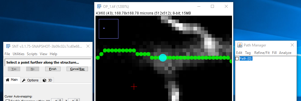
To force the start of the new path to be a branch of the selected path, hold down the ⌥ Alt + ⇧ Shift keys while you move the mouse to find the branch point under the red cross-hairs, now decorated with a “Fork Point” annotation. With ⌥ Alt + ⇧ Shift held down, click with the left mouse button. Finally, release the keys.
 NB:
NB:
- It is also possible to zoom into the branch point, right-click on the image and choose Fork at Nearest Node from the contextual menu
- The forking shortcut can also be simplified (Temporary Paths section of the Options tab)
III. Extend The Path
From this point on, you can carry on adding nodes to the branched path as above, i.e., Create a temporary path and confirm it. When you decide to complete the path you should see in the Path Manager that it has been recorded as a child of the existing path.
Accurate Point Placement
You can follow these instructions using File › Load Demo Dataset… and choosing the Drosophila OP neuron (Complete 3D reconstruction) dataset. All the neuronal processes are traced in this dataset, so you may want to delete some of the existing paths beforehand.
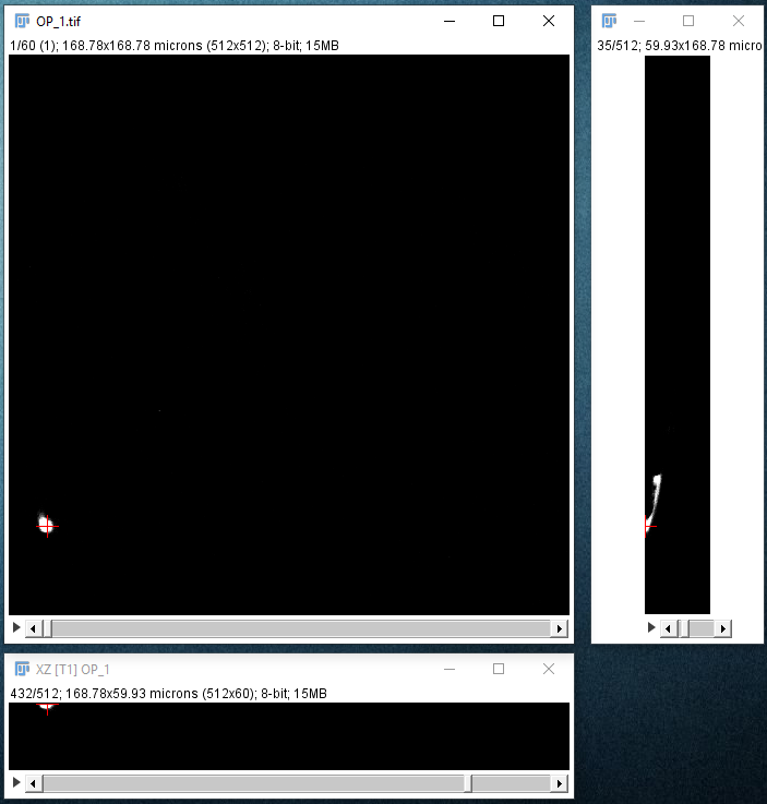
Accurate node placement requires XY, ZY and XZ views to be visible. You can do so at startup, by making sure that Default: XY, ZY and XZ views is selected, or by clicking in Display ZY/XZ Views in the Options tab if you have already started SNT.
|
Find the approximate location of your start point by moving your mouse in the XY window, holding down ⇧ Shift to synchronize the view in the other panes. At this point, you should enable cursor auto-snapping in the Main tab using suitable parameters for your image. When this option is enabled, the cursor will automatically 'sniff' for local maxima and 'snap' to their average X,Y,Z position. The pixel that is most likely to be on a neurite is indicated by the red cross-hair cursor. |
|
|
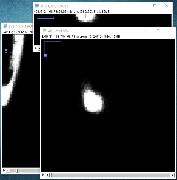
When you press + to zoom in, all the panes will zoom in on the point that the crosshair is over, so each time you press +, make sure you move your mouse pointer over the neurite so that it's still over the structure of interest. You may want to adjust in the Views widget (Options tab) whether all views should zoom synchronously. Note that when Z-snapping is enabled, all views become synchronized |
|
|
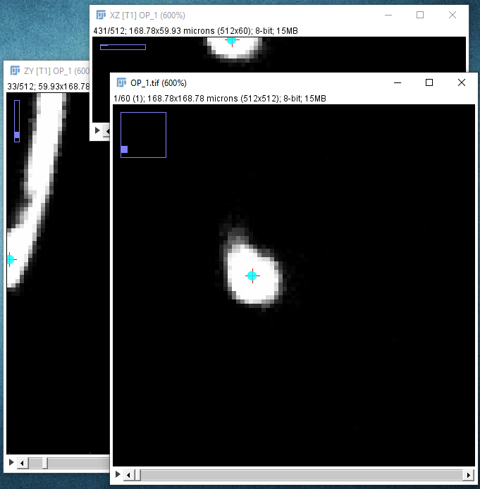
Locate the center of the structure to be clicked on. If cursor auto-snapping is enabled, simply mouse over the structure, otherwise, try moving the mouse and scroll wheel in each of the panes (holding down ⇧ Shift to synchronize the views in all three panes). Note that you can toggle the cursor auto-snapping feature at will, by pressing the shortcut S. Also, note that you can "click" on the brightest voxel of a voxel column, by pressing M. When you're happy with the point under the crosshairs, left-click to start the path: |
|
|
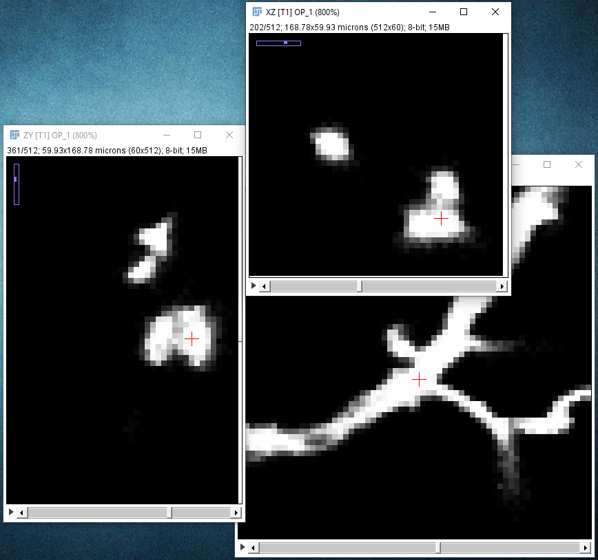
Zoom out again with the - key, and similarly zoom in on the next point you want to be on your path to place it precisely: |
|
|
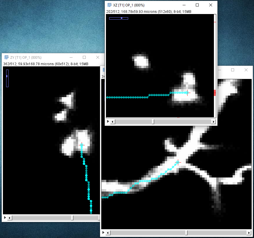
The path along the neuron may not follow the center line perfectly: |
|
|
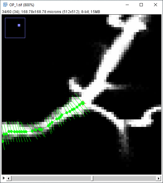
... but you can later improve that with the Refine/Fit › Fit Path... option in the Path Manager, which tries to align the path to the midline of the structure to sub-voxel accuracy: |
|
Tracing in the Legacy 3D Viewer
The legacy 3D Viewer allows for tracing in an interactive 3D scene.
By default, the Legacy 3D Viewer displays warnings and errors in pop-up dialogs. If you find this distracting, you can toggle Quiet mode (log errors to Console) to have them displayed in a non-blocking Log window.
I. Starting the Viewer
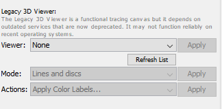 To open the viewer, select the 3D menu tab in the SNT dialog and look for Legacy 3D Viewer. You will see several parameters:
-
Select New with image… from the Viewer drop-down menu and press Apply. Note that you can re-use existing viewers you may have open by choosing their window titles from the drop-down menu. NB: Selecting New without image would only allow you to look at reconstructions without the underlying signal.
-
Large images may require downsampling for performance reasons. Once you Apply the viewer choice, a prompt will appear asking you to choose the downsampling factor for the image. E.g., a value of 2 means here that the image is downsampled by a factor of 2 in x-, y- and z-direction. Note that while downsampling speeds up rendering it often results in signal smoothing. Volumes should look crisper without downsampling. Original pixels are used with a resampling factor of 1.
-
Once the downsampling factor is specified, the viewer window will appear with the currently open image (i.e., the current Channel/Frame being traced as specified in the Data Source widget).
-
Options in the Mode drop-down menu specify how paths should be rendered. There are three possibilities: 1) Lines: Only the centerline of paths is displayed; 2) Lines and disks: Centerline of paths is displayed with disks at each node depicting the node radius; and 3) Surface reconstruction: Paths are displayed as surface meshes.
It is recommended to render color coded paths in either Reconstruction Plotter or Reconstruction Viewer because the algorithms that allow paths to be mapped to lookup tables have not been ported to the Legacy 3D Viewer.
II. Tracing and Navigation
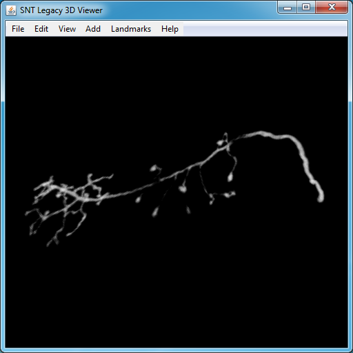
Selecting points for tracing
Tracing mode is only active when the Wand tool in the main ImageJ toolbar is active. To activate it, press the W (shortcut) and click over the region you want to trace. Tracing works the same way as in the XY, YZ, and XZ views, i.e., click somewhere in the image to create a starting point, then click further along the structure of interest to find a path between the two points, then confirm or deny the temporary segment as described above. Similarly, branching occurs as described for 2D canvas(es), by holding the ⌥ Alt + ⇧ Shift modifier. NB: This shortcut can be simplified: See Options Tab for details.
To interact with the scene without tracing, activate the Hand tool in the main ImageJ toolbar by pressing H.
Navigation
-
Rotation: Use
Middle Drag. Alternatively, if the Hand tool (H) is active in the ImageJ toolbar you can use
Left Drag
-
Translation: Use ⇧ Shift +
Middle Drag. Alternatively, if the Hand tool (H) is active in the ImageJ toolbar you can use ⇧ Shift +
Left Drag
-
Zoom: Use
Mouse Wheel
See Key Shortcuts for the list of all supported shortcuts.
Note that the 3D Viewer is not aware of commands listed in the Image Contextual Menu (e.g., Path Editing). Such commands need to be accessed from the image canvas
Merging/Joining Paths
You can follow these instructions using File › Load Demo Dataset… and choosing the Drosophila OP neuron (Complete 3D reconstruction) dataset. All the neuronal processes are traced in this dataset, so you may want to delete some of the existing paths beforehand.
Two paths can be merged or joined in Edit Mode. To do so:
- Select a path and enter Edit Mode (by right-clicking on the image canvas to access its contextual menu)
- Activate the node to be merged by hovering over it
- Select the second path by using the G shortcut and activate the second merging node by hovering over it
- Open the contextual menu and select the initial path from the Connect To (Start Join) / Connect To (End Join) menu
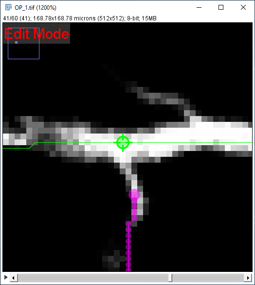
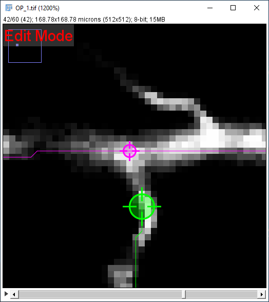
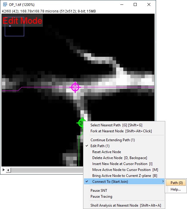
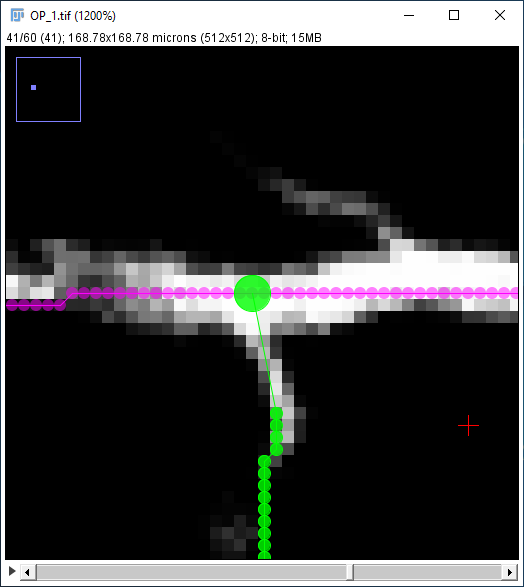
Important Notes:
- If both nodes are terminal, the paths are merged together. Otherwise, one path will become a child of the other. Note that one of the nodes must be terminal, to ensure no loops are created.
- The direction of merge matters, and it is assumed to be always from parent to child. If the child path is oriented in the wrong direction (i.e., moving “towards” its parent at the point of merge), it will be re-oriented so that single root connectivity is maintained
- Loop-forming connections are not allowed
- The recommended way to concatenate or combine paths is to use the respective commands in Path Manager’s Edit menu
Use Path Orientation (hold O) to verify path orientations before merging.
Full-automated Tracing
Described in Auto-tracing.
Spine/Varicosity Analysis
Described in Spine/Varicosity Analysis.
Delineation Analysis
Described in Delineation Analysis.
Time-lapse Analysis
You can use one of two demo datasets (File › Load Demo Dataset…) to follow these instructions:
- Hippocampal neuron (DIC timelapse) dataset: A timelapse video of a cultured neuron in which neurites have been pre-traced across time
- Segmented video (2D timelapse) dataset: A small, thresholded video of a cultured neuron processed by a script that automates tracing at each frame
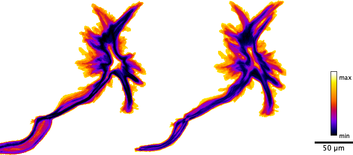
Mitigation of motion artifacts. Left: Projection of inter-frame differences across the original time-lapse sequence. Right: Inter-frame differences of the same time-lapse after 3D drift correction. Neurite displacements are color coded with warmer hues indicating higher motility. Note how lateral motion around the soma and along the longest extending neurite (lower left) has been minimized. Hue ramp has been scaled to the smallest (min) and largest (max) displacements in the sequence.
The first step is to ensure that the time-series is not affected by artifactual motion. Fiji features a host of registration tools to mitigate such artifacts. Arguably, one of the most intuitive of such tools is Correct 3D Drift because it can correct abrupt displacements as well as slow drifts.
SNT features Scripts › Time-lapses › Apply 3D Drift Corrections…, a convenience wrapper for Correct 3D Drift that applies drift correction to the image being traced, as well as existing paths. However, if your time-lapse video is rather large it is recommended that you run Correct 3D Drift (or alternative registration routine) before loading the image in SNT to avoid running out of RAM. The illustration on the right highlights the type of mitigation you should expect.
Once undesired motion has been mitigated:
-
Specify the first time-point to be traced using the Data Source widget
-
Trace the path of interest. This can be done manually or perhaps automated via a script (see below)
-
Repeat 1. and 2. for all the frames to be traced. There are a couple of ways to expedite tracing across frames:
-
Duplicate the path(s) of interest using Path Manager’s Edit › Duplicate… This will allow you to copy a path (and its children) to a new frame (or channel). If a neurite is retracting, you can duplicate the subsection of the path that better matches the retracted neurite: e.g., by restricting the duplication to a fraction of the path’s total length, or up to a branch-point
-
Use a script to attempt segmentation at each frame, as in the Segmented video (2D timelapse) demo (File › Load Demo Dataset…)
-
-
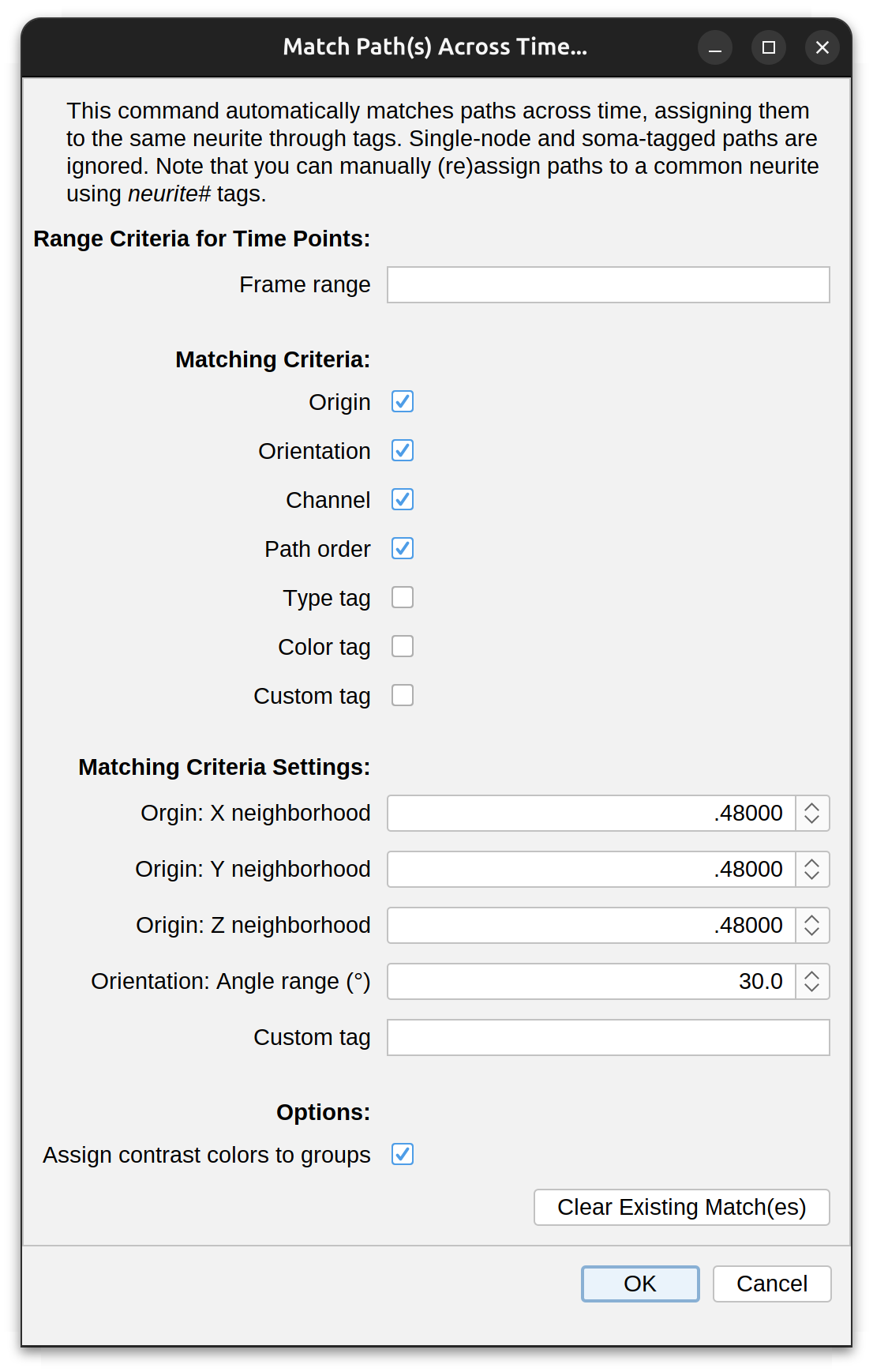
Run Path Manager’s Analyze › Time-lapses › Match Path(s) Across Time…. The dialog allows you to match paths in the same time-series to a common neurite. Note that the command matches only selected path(s) (or all paths if no selection exists), but ignores Paths tagged as ‘soma’. Options include:
-
Frame range Only paths associated with these frames will be considered for matching. Range(s) (e.g. 2-14), and comma-separated list(s) (e.g. 1,3,20,22) are accepted. Leave empty or type all to consider all frames
-
Matching criteria These are a series of conditions that matching paths must fulfill. Some require no further adjustments (e.g., channel, path order, type tag, color tag) while others have configurable settings. Criteria can be combined E.g., if channel and type tag are selected, paths need to share the same channel and the same type tag (‘Axon’, ‘Dendrite’, etc.) to be matched.
The criteria with configurable settings are perhaps the most commonly used:
-
Starting node location If selected, matching paths need to share a common origin (starting node) in terms of (X, Y, Z) coordinates. Sample movement and focus drift are common during time-lapse sequences. To account for this, it is possible to specify a (X, Y, Z) ‘motion-shift’ neighborhood: Paths that originate within this neighborhood (in spatially calibrated units) are considered to share the same starting node location
-
Orientation If selected, paths need to extent under the same overall direction (outgrowth extension angle) to be matched. Paths sharing an outgrowth angle +/- the specified range (in degrees) are assumed to share the same overall direction of growth
-
Custom tag If selected, matching paths need to share the specified (case-sensitive) tag. A regex pattern can also be specified
-
-
NB: Note that any mistakes by the matching algorithm can be corrected by editing neurite# tags manually
-
-
Once paths have been matched to their neurites across the time-lapse sequence, future analysis becomes simplified.
-
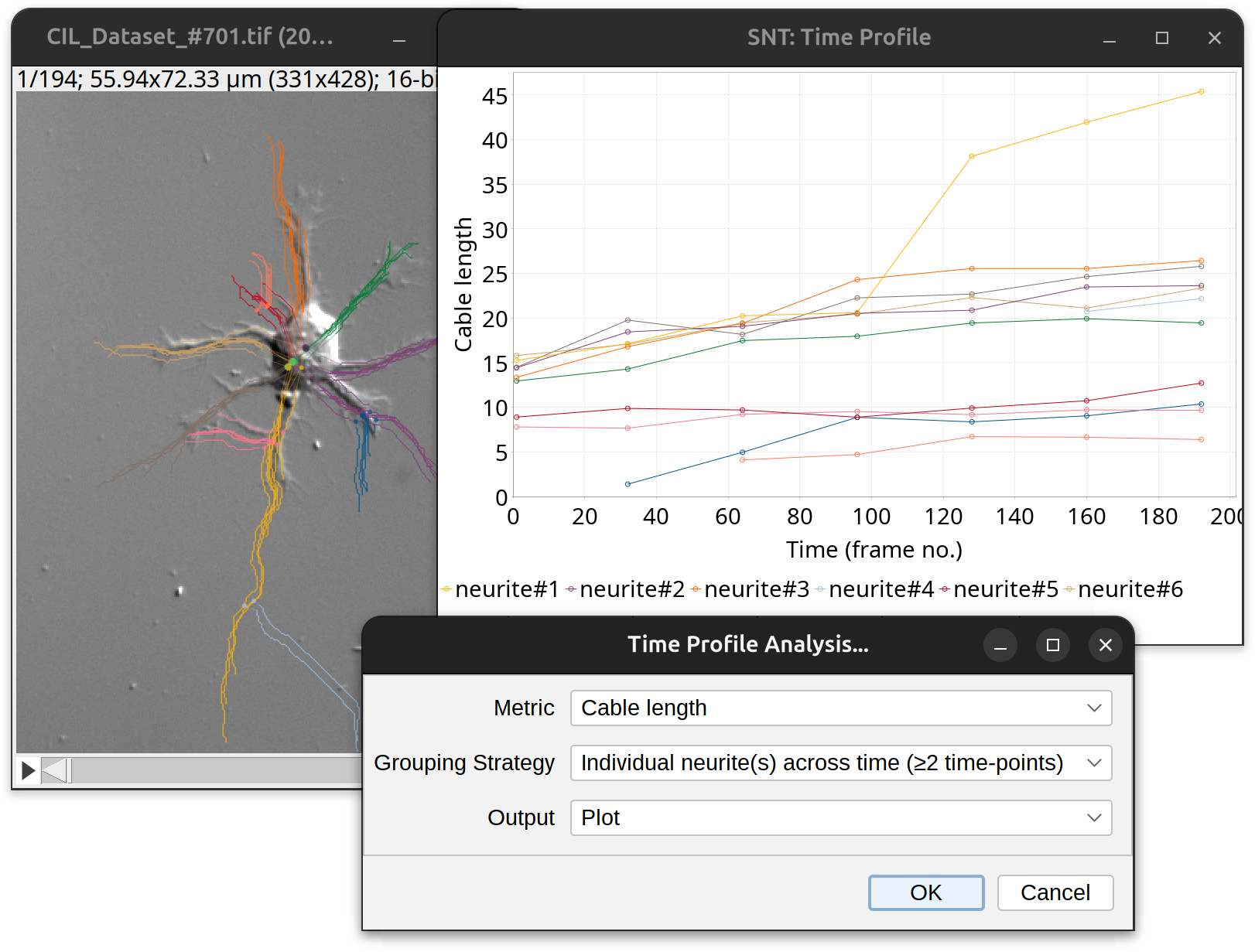
Use Either Analyze › Time-lapses › Grow Analysis… or Analyze › Time-lapses › Time Profile… to analyze the data. The former is a very simple approach to summarize growth across time, while the latter is a comprehensive analysis tool. Time Profile… includes the following options:
-
Metric the measurement to be profiled across time
-
Grouping strategy Typically this would be set to Matched path(s) across time to reflect the matching performed in 4. However, if there are many short-lived neurites (i.e., only visible in few frames) it may be beneficial to choose Matched path(s) across time (≥2 time-points). This will only consider paths present in two or more frames. A no grouping strategy is also available for cases where step 4 was skipped.
-
Output Whether a plot, a table or both should be created
-
-
For more complete, thorough measurements, use Grow Analysis: In addition to growth trajectories, this option classifies motion growth phases, including elongation and retraction events, phase transitions, angular velocity changes, and directional steering.
Filling
You can follow these instructions using File › Load Demo Dataset… and choosing the Drosophila OP neuron (Complete 3D reconstruction) dataset.
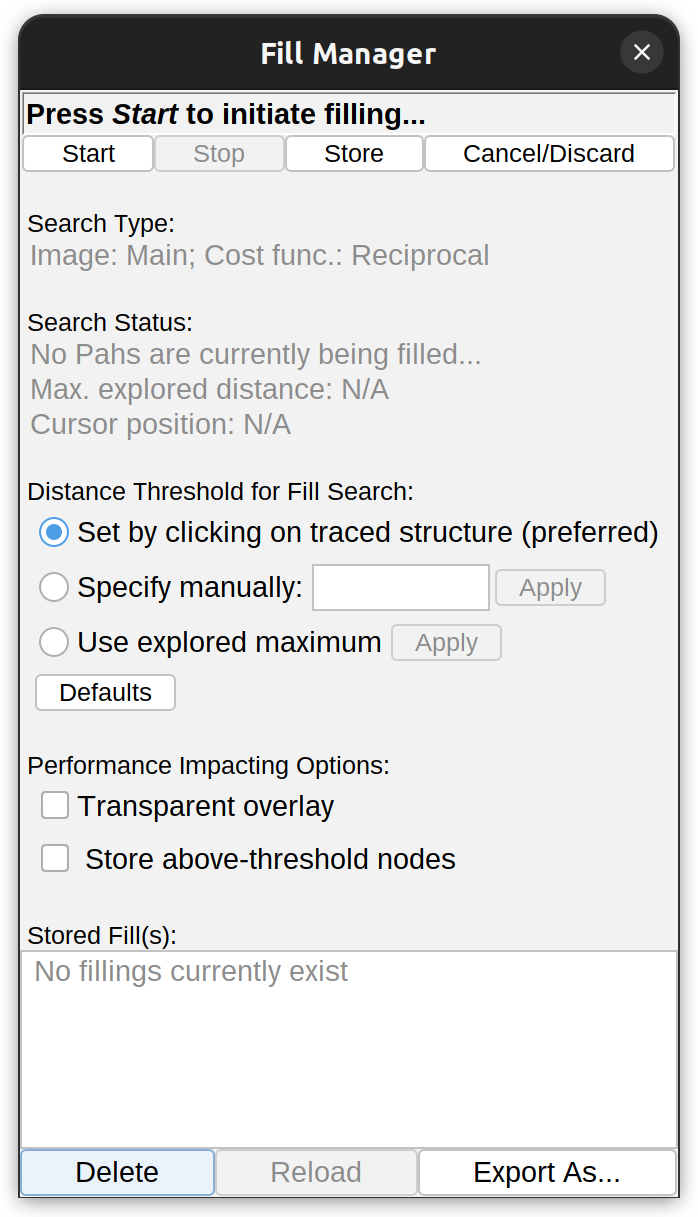 Paths can be “filled out” to volumes, i.e., converted into 3D images that can be used to improve the visualization of the shape of a neuron beyond what can be seen from traced center-lines, and/or subsequent image processing routines. The filling algorithm uses the center-line path coordinates as seeds in a ‘signal search’ that expands along neurites to encapsulate the neurite in 3D. The result can be exported as different types of images, including distance maps, binary masks or labeled image.
Fillings are controlled by the Fill Manager and share many of the same properties of auto-tracing:
-
Fillings can be performed on the main image or secondary tracing layer
-
The same cost function used in auto-tracing is used for filling
-
Fillings will be more accurate once SNT is aware of properties of the image being traced, so before filling imported paths you may need to re-trace a representative neurite (you can discard the result)
I. Starting the Fill
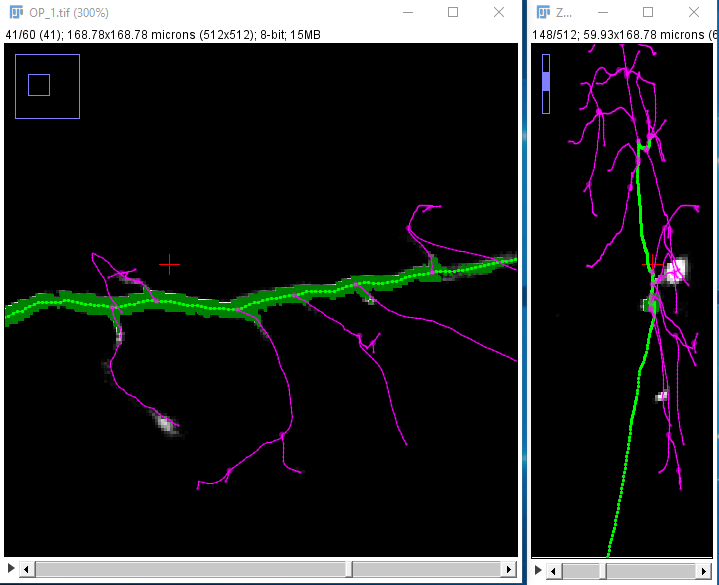
First, select the one or more paths that you want to fill out from in the Path Manager and select Fill › Fill Out… in the Path Manager (or select none if you want to fill all the existing paths). Once the filling starts, you should be able to see a thick green surround the path while scrolling through the 3D stack:
The filler continues to explore the image until you click “Pause” or “Stop” in the dialog, or until all the image has been fully explored. However, the fill which is shown only includes those points up to a certain threshold distance from the path. Note that this “distance” doesn’t mean a real physical distance, but instead a ‘likelihood-distance’: a measure which takes into account the intensity values of the pixels which must be passed through when moving away from the path. Information about the current threshold and the progress of the search is shown in the dialog. Note that if your image is rather small, the entire image may be fully explored before you have time to interact with prompt.
 The “Cursor position:” state under “Search Status” is updated as you move your mouse over the image. If the point under the mouse has been reached by the search then it will show you that point’s distance from the path. Otherwise, it will read “Not reached by search yet”.
The Search status shows your current threshold distance: so if this is set to 0.2 then that means that all points less than 0.2 from the path are included in the fill (and highlighted in green in the image). The “Max. explored distance:” shows the maximum distance from the path that has been completely explored.
II. Adjusting the Fill Threshold
You can change the fill threshold in one of three ways:
-
Clicking on a point in the image that has been reached by the search (This is the most intuitive way of altering the threshold). It may be helpful to disable the “Enable Snapping within: XY-Z” feature for the cursor while doing this
-
Manually changing the threshold in the “Specify manually:” input box and clicking the “Apply” button beside it.
-
Clicking the “Use explored maximum” button below the threshold input box and click “Apply”, which sets the threshold to the maximum explored distance (the value shown in “Max. explored distance:” under the “Search Status” dialog).
We will assume that you want to use the first of these approaches:
-
It is difficult to set the threshold accurately from the image unless you zoom in, so first zoom on part of the path that you want to set the threshold for.
-
Since the solid green fill obscures the intensity value of the points in the fill, you may want to activate the Transparent overlay checkbox. Note that this could slow down filling, although the performance hit is usually negligible.
-
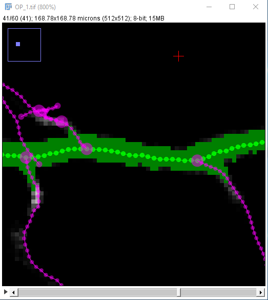
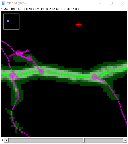
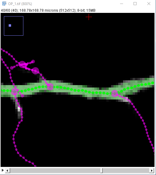
As you can see in the middle image, the threshold is set too far from the path, since there are many background voxels under the green fill, as well as voxels on different paths than those of interest. Experiment with clicking on different locations closer to the path in order to adjust the threshold until you are satisfied with the result. You might end up with something like the rightmost image:
III. Understanding Fill Distances and Distance Threshold
Fill distances should be interpreted as ‘likelihood distances’:
Voxels associated with low distances are likely associated with the traced path. Voxels associated with high distances are unlikely to be associated with the path.
The smallest distance corresponds to a perfect match to whatever information the filler has on the center-line of the traced path, and the highest distance correspond to the worst match. When a threshold is set, pixels are clustered into two groups: those that ‘fill’ the path and those above threshold that don’t.
Note that likelihood distances are under an arbitrary range. Consider a scale ranging from ]0 to 1]: If the threshold distance is set at 0.2, paths are only ‘filled’ with voxels that share at least 80% likelihood with the traced center-lines. In practice, the upper limit of this distance depends on much of the image has been explored by the algorithm. Thus, it is not trivial to define a priori a sensible threshold. It should be assumed that the range of possible distances falls between 0 (perfect likelihood, i.e., center-line voxels themselves) and a maximum corresponding to the most distinct voxel to the path center-line. Such voxel of “maximum difference” is expected to belong to the image background (unlabeled neurite). Distances can be studied by exporting fills as Distance maps.
While adjusting the distance threshold is the single most effective way to improve ‘fills’, other approaches can also improve the result:
-
Adopt secondary layers: Currently, the filler only looks at pixel intensities, and thus likelihood is a simple comparison of gray value intensities, but note that other features can be used by the algorithm, when a secondary tracing layer is used. E.g., If the filling occurs in a Tubeness flavor of the image, then distances reflect likelihoods of association with tube-like structures.
-
Optimize center-lines: Since center-line pixels function as seeds, ensuring they follow closely the curvatures of the fluorescence signal using Path fitting may improve the result
IV. Completing the Fill
If the search is still active, you might as well click “Pause” so halt exploration of the image. Then you can either:
-
Save the fill (which will add it to the fill list) by clicking “Store”
-
Discard the fill by either clicking “Cancel/Discard” while filling is in progress or, if you stashed the fill, select it in the fill list and click “Delete”
V. Exporting
-
The “Export” button provides several export options, including:
-
Binary mask: Only the points in the fill are preserved under a constant value. This is useful to e.g., mask out structures outside the neuron being traced, or to train a TWS/Labkit model.
-
Grayscale: Only the points in the fill are preserved under the original pixel intensities. This is useful to e.g., render the structure in the legacy 3D Viewer or sciview to do a surface rendering of the neuron.
-
Labels: Each group of paths (Tree) gets assigned a unique pixel value so that such groups are distinguishable from each other. Note that scripting can be used to extend this option to individual paths so that each path in a group gets assigned a unique label (see the Fill_Demo.py script and this discussion for details)
-
Annotated Distance map: Points along the fill are assigned the explored distance as described earlier. Useful for debugging and/or perusing the fill operation
-
CSV export: Exports details of the filling operation as tabular data. This includes distance thresholds, algorithms used, and volumes of filled paths
-

Currently, only the output images/CSV summary of fills are exported. TRACES files contain only the search parameters of fill operations which allows SNT to recapitulate the search when files are reopened. No information on fills is stored in SWC files.
Detecting Crossovers
Described in Curation.
Generating Filtered Images in Bulk
This section describes how to generate Filtered Images outside SNT in bulk. Note that there are many tutorials on this topic. Arguably, the easiest way to process multiple images is to 1) record a macro that processes a single image, then 2) wrap it in a loop to iterate over all files in a directory. For example, using IJ1 macro language:
d = getDirectory("Select a directory");
files = getFileList(d);
extension = ".tif";

for( i = 0; i < files.length; ++i ) {
    filename = files[i];
    if( endsWith(filename,extension) ) {
        l = lengthOf(filename);
        el = lengthOf(extension);
        basename = substring(filename,0,l-el);
        expected_window_name = "result";
        output_filename = d + File.separator + basename + ".tubes.tif";
        open(filename);
        run("Gaussian Blur...", "sigma=2 scaled stack"); // processing step here
        selectWindow(expected_window_name);
        saveAs("Tiff", output_filename);
    }
}
The same process can be accomplished more completely in a script using ImageJ Ops. For example, in Jython:

](/media/plugins/snt/snt-growth-analysis.png)