Deconvolution corrects the systematic error of blur (loss of contrast in smaller features) in optical systems such as fluorescence microscopy images.
The problem, and the solution
Any optical image forming system, such as a microscope objective lens, has the nasty property of killing more and more contrast of smaller and smaller features, up to the resolution (diffraction) limit, after which there is no contrast (and thus no resolution). Large features are bright, but small features appear less contrasted and dimmer than they should. This is a systematic error, characterized by the Point Spread Function (PSF) of the optical system, which makes the image intensity information non-quantitative. If we can measure the PSF, or guess it, we can correct the raw image for it. Since it’s possible to correct such a systematic error, we should!
Image contrast restoration by deconvolution is a way to correct the systematic error of contrast loss in an image recording system, such as a microscope objective lens or telescope mirror or lens. We try to reverse the effects of blur in the recorded image, caused by convolution (blur, smearing, loss of contrast of small features) of the real image due to the imaging point spread function (PSF).
Image contrast restoration by deconvolution is an important systematic error correction step for quantitative measurement of image pixel intensities in analysis workflows. If we don’t correct this systematic error, the results of the image intensity analysis could be very much more wrong than if we correct the images before analysis. It’s the same as zeroing a scale before weighing something.
Introduction to the practical method
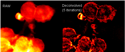
Two plugins from Bob Dougherty can be used together to perform this systematic error correction in a 2D or 3D image. Other plugins are also available. The Diffraction-PSF-3D plugin generates a z-stack of the theoretical point-spread function (PSF). Alternatively, an empirical, measured PSF could be used. The Iterative Deconvolution 3D plugin uses a PSF image z-stack to correct the image contrast vs. feature size in your sample image z-stack. The image below is a single slice taken from a stack before and after deconvolution using these plugins.
See the plugins’ homepages for more details: Diffraction PSF 3D & Iterative Deconvolution 3D
Generating a PSF image stack
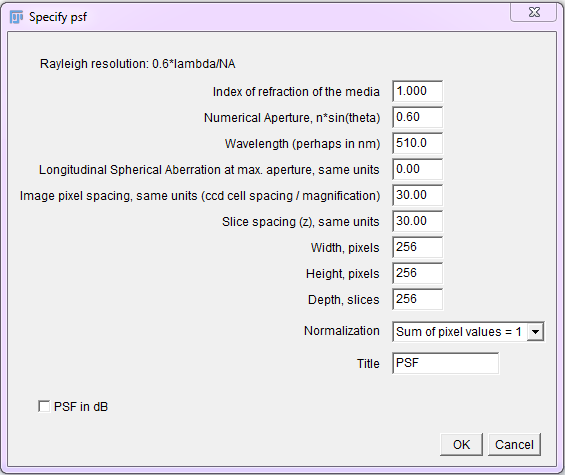
The Diffraction PSF 3D plugin can be used to generate theoretical PSFs assuming they arise only from diffraction. These PSFs may be used with other deconvolution plugins later.
To use, run the “Diffraction PSF 3D” plugin. A dialog will appear; most of the fields are self explanatory. The width, height and depth values are for the PSF image, not your image stack. The desired values will need to be empirically determined. Try to match the parameters used to capture the raw image.
Constrained Iterative Deconvolution
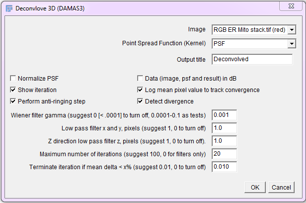
Non negative constrained (non linear), iterative deconvolution algorithms greatly outperform simple inverse filters and Wiener filters on noisy real life fluorescence microscopy (and other) image data.
Run the Iterative Deconvolve 3D plugin, then select the image and PSF. For a 2D image, use a 2D (single plane) PSF. For 3D images, use a 3D PSF (z stack). Start with the default values and set iterations to 10 initially. Be careful not to run out of memory when processing large 3D images. Crop them if they are too large.
An interactive Convolution / Deconvolution / Contrast Restoration demo in ImageJ
For an educational interactive ImageJ javascript demo of convolution, inverse filtering and image contrast restoration by iterative constrained deconvolution (using the above plugins), see this Convolution / Deconvolution / Contrast Restoration demo script
Video presentations
Tips and how-tos
Compiled by E. Crowell and D. J. White
What the hell is the point spread function (PSF) and why should I care?
The PSF is the image of a point source of light as imaged through a lens (or set of lenses). It is the function (shape) describing the diffraction of light in an optical system. For microscope systems, it can be derived from processed images of sub-resolution fluorescent beads, or an approximation can be calculated from optical theory equations.
Three different types of PSF images are useful:
- The raw measured PSF obtained by imaging sub-resolution size beads using the optical system.
- The measured PSF obtained by acquiring and processing multiple z-stacks of sub-resolution size beads.
- The theoretical PSF generated by a computer program, after input of values describing the optical system.
It is necessary to measure the PSF of the optical system to verify that no abnormalities are present. Imaging sub-resolution beads is a sensitive method to detect any problems in the optical system. If the Airy rings in the raw PSF are highly asymmetrical, it indicates a problem, such as an objective lens that might be fractured, scratched, misaligned, or simply dirty. Another possibility is that the coverglass could be at an angle rather than being exactly flat.
The effective numerical aperture (NA) of the objective can also be estimated by measuring the angle of the cone of light in the raw PSF. If the raw PSF has the expected characteristics of a good quality optical system, then a theoretical PSF can be used for deconvolution and the time-consuming processing steps to generate a useful measured PSF (see below) might be avoided. However, since no optical system is perfect, a high-quality measured PSF will typically give better results than a theoretical PSF.
A normal measured PSF image consists of a three-dimensional Airy pattern of rings of increasing diameter which radiate out from a spherical bead as one increases or decreases the z-position. The Airy rings should be radially symmetrical circles if the lenses are in good condition. When viewed orthogonally, two cones of light are visible around the fluorescent bead (point source of light). The cones of light will not necessarily be perfectly symmetrical in the z-axis, depending on the quality of the optical system. This asymmetry is one characteristic of the measured PSF which makes it superior to the theoretical PSF for deconvolution applications. A very asymmetric PSF in z is indicative of the presence of spherical aberration, due to wrong coverglass thickness and/or refractive index mismatch between the sample mounting and lens immersion media.
In order to successfully measure the PSF, the fluorescent object being imaged should behave as a point source of light. For this to be possible, the fluorescent beads should be smaller than the optical resolution of the system (e.g. 100 - 170 nm diameter). The optical resolution = 0.61 . lambda / NA , where lambda is the emission wavelength of the fluorophore and NA is the numerical aperture of the objective. All things being perfect, a 1.4 NA objective has an optical resolution of ~ 250 nm. In optimal conditions, the pixel spacing in the digitized image should be 2.3-3 times smaller, in the range of 80 - 100 nm or a bit less, to fulfill the Nyquist - Shannon sampling criterion and to avoid missing information, over-sampling, or under-sampling.
Fluorescent beads larger than the optical resolution do not behave as point sources and deform the light passing through them due to their refractive index being higher than that of the mounting medium.
Before acquiring z-stacks to generate a measured PSF, one should consider the acquisition conditions that will be routinely used to generate images for deconvolution. The measured PSF image should be sufficiently sampled so that no information is lost, yet must be of dimensions that are equal to (or smaller than) the dimensions of the images to deconvolve. The PSF image must “fit” into the image to deconvolve. The PSF image should be large enough in xy to accomodate the full Airy rings, and large enough in z to make the cones of light visible and complete.
The PSF shape depends on three criteria:
- The emission wavelength of the fluorophore
- The objective used (magnification and NA)
- The refractive index of the objective lens immersion medium
For proper deconvolution, the z-step interval is also an important factor, since the PSF image and the z-stack to be processed should ideally have the same z-step interval. PSF images with a smaller z-step interval than that of the z-stack to be processed can also be used.
Therefore, a distinct PSF must be acquired/created for every combination of these criteria routinely used when acquiring images.
Post-processing of acquired PSF images to generate a measured PSF
A high-quality PSF image is difficult to generate by acquiring images of sub-resolution fluorescent beads. Such small beads seldom contain enough fluorescent dye to yield a high signal-to-noise (SNR) ratio. Therefore, z-stacks should be acquired using a relatively high exposure time (> 200 ms). Caution should be used to avoid increasing the exposure time or lamp power to a level which will cause rapid photobleaching of the bead. If photobleaching occurs during acquisition of the PSF z-stack, it will result in a false PSF due to loss of signal caused by photobleaching.
The beads should be sufficiently diluted so that on average only one bead is visible per field of view. (Neighboring beads will contribute their own light diffraction patterns and deform the measured PSF.) Appropriate beads for measuring PSFs should have a low tendency to aggregate. Nevertheless, with subresolution size beads, one can never know if one is imaging a single bead, or a pair or small cluster of beads. Therefore, it is necessary to image multiple fluorescent beads and to compare the obtained PSFs. The ones that show nicely symmetrical Airy rings represent the useful PSFs. If none of the PSFs obtained shows the expected pattern, there is likely a problem in the optics (see above).
A PSF should be obtained for every combination of z-step intervals, wavelengths, objectives, and immersion medium. However, there is no sense in measuring the PSF of low magnification objectives which give undersampled images, or stainings like DAPI which do not need to be deconvolved.
The last step in generating a useful measured PSF for deconvolution is to subtract the background signal from the stacks so that some pixel values will be equal to zero where there is no real signal. To accomplish this, simply measure the mean intensity of a black region in the stack, outside of the Airy rings. This mean value represents the background signal in the image, which usually originates from the positive offset/bias of a CCD camera chip. Subtract the mean value from all the pixels in the stack (use ImageJ › Process › Math › Subtract…). If this step is omitted, square deformation artifacts may be visible in the deconvolved image.
Obtaining images optimized for deconvolution
It is best to start the z-stack well above the object of interest, and to continue well below, in order to cover the PSF of every interesting point in the sample. If only the “in focus” part of the sample is imaged, the deconvolution result will not greatly improve the image since information is missing.
The appropriate z-step interval can be calculated from the Abbe/Rayleigh diffraction limit equation \(Dz = {(lambda \times RI) \over (NA \times NA)}\) where Dz = the ideal z-step interval in nanometers, lambda = the emission wavelength, RI = the refractive index of the mounting medium, and NA = the numerical aperture of the objective. For example, a z-step interval of ~ 350 nm is appropriate for imaging FITC fluorescence using a 1.4 NA objective and a mounting medium with an RI of 1.5.
Always use the same conditions that were used for acquisition of the measured PSF, or generate a theoretical PSF that corresponds to your exact conditions.
How to do the deconvolution
Several plugins for imageJ exist. The most sophisticated are the DeconvolutionLab (BIG - EPFL) and the parallel iterative and spectral deconvolution plugins.
For further very nicely written and informative descriptions of this topic, see the Huygens deconvolution guide.