This page describes a detector module for TrackMate that relies on StarDist to segment objects in 2D. It is not included in the core of TrackMate and must be installed via its own update site.
Installation
You need to subscribe to several update sites:
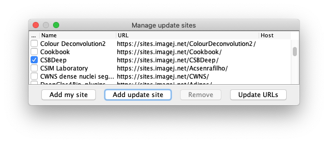
- the CSBDeep update site,
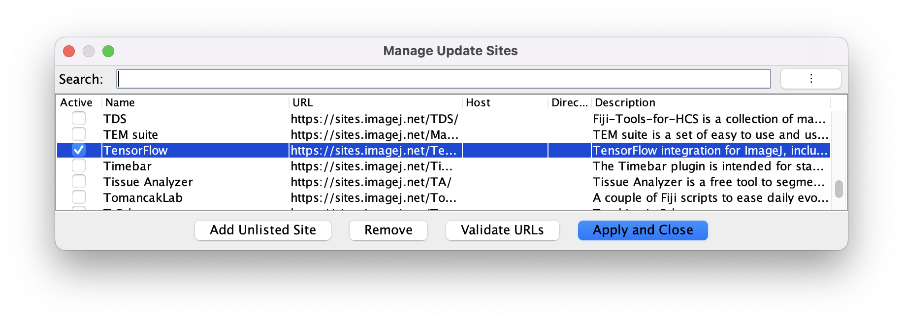
- the Tensorflow update site,
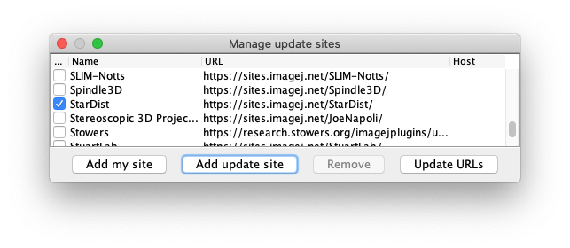
- to the StarDist update site,
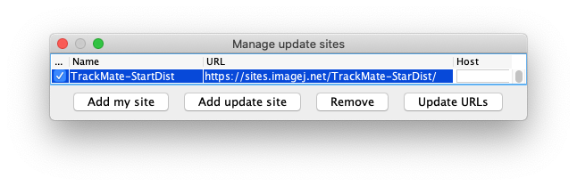
- then to the TrackMate-StarDist update site:
The CSBDeep update site:
The Tensorflow update site:
The StarDist update site:
And finally the TrackMate-StarDist update site.
Once you have them all, please restart Fiji. We suggest that you test StarDist by itself just to make sure it runs after installation. This way we can better find what is wrong in case it does not work. Follow for instance the instructions on the StarDist page.
Usage and tutorial
TrackMate-StarDist ships two detectors that will appear in TrackMate. After installing TrackMate-StarDist and restarting Fiji, these two detectors will be integrated in TrackMate in a transparent manner. We describe how to use them in the four tutorial below. They describe in order:
- Using TrackMate-StarDist on a single-channel image.
- Using TrackMate-StarDist on a multi-channel image and exploiting the intensity information.
- Using TrackMate-StarDist with a custom Deep Learning model.
- Using TrackMate-StarDist to segment a 3D image using a slice-by-slice approach.
StarDist detector with builtin versatile nuclei model on a single channel image
The StarDist plugin comes with a very efficient model that can segment nuclei imaged in fluorescence in 2D, generated from the dataset in the Kaggle challenge of 2018:
We use this model in the first StarDist detector.
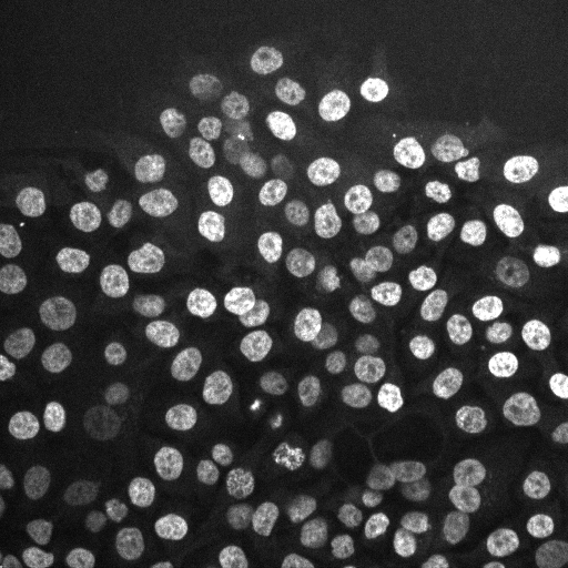
In the first tutorial we will use a movie following the migration of cancer cells, labelled for their nuclei. You can download it from Zenodo:
![]()
First launch Fiji and open the tutorial image in Fiji.
We use here the P31-crop.tif file, provided in the tutorial data.
Then launch TrackMate Plugins › Tracking › TrackMate.
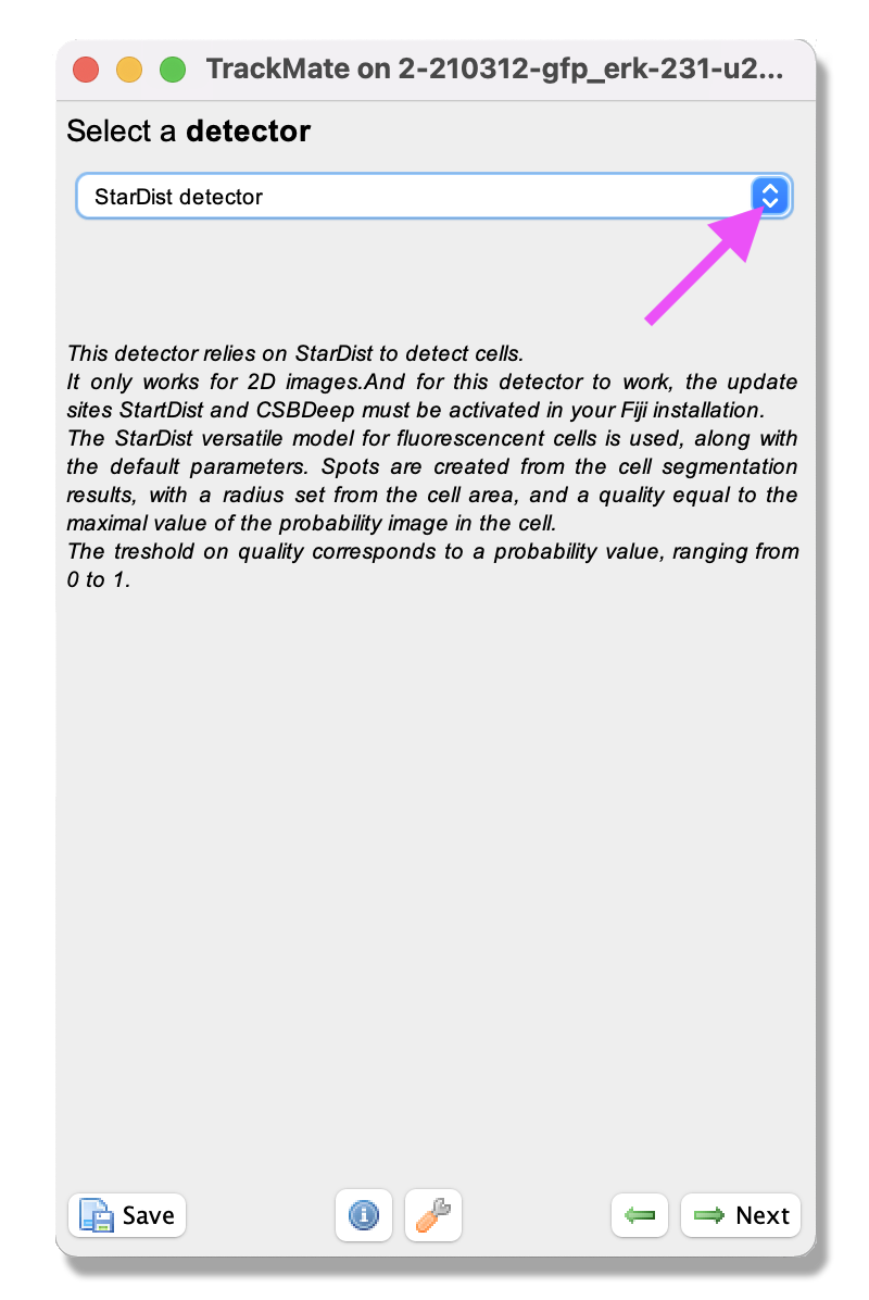
In the second panel titled Select a detector, you should see two new choices in the list, and on of them is StarDist detector.
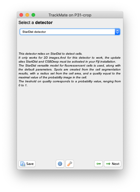
Select it and click Next.
This simple panel appears.
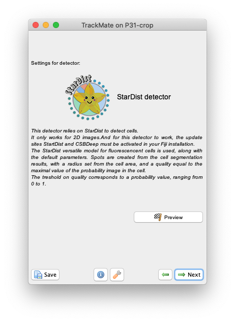
Note that in this panel there is no configuration for Stardist detector: we use the default values of this model for the score threshold and overlap threshold. We observed, that in cases when this model with the default values does not work well with some dataset, changing the score and overlap threshold have little to no positive impact on the results. We reasoned therefore that if the model and the default values do not work well for your data, it is best then to train a specific StarDist model for your problem.
Check the results of segmentation by clicking on the Preview button.
Here is what I get on the first time-point of the tutorial image:
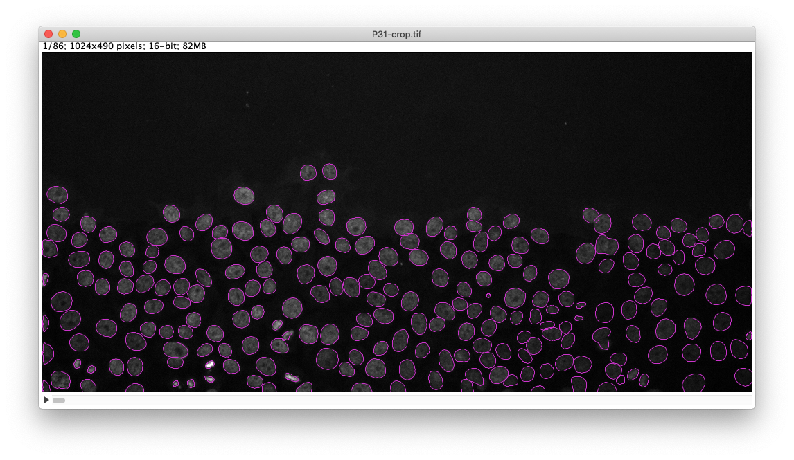
The StarDist model works really well with this kind of data. After that you follow through the next steps in TrackMate to segment all cells in all time-points then track them. Using the default tracker and default parameters each time we get this result:
It was simple and fast, which means that careful inspection for missed cell divisions and false links is on order.
ERK signalling and motility assay with a multi-channel image
In this part of the tutorial we will correlate the translocation of an ERK reported in the nuclei with cell motility. We will use images from a cell migration assay, where cells are expressing an ERK reported in the first channel, and are stained for their nuclei in the second channel. The analysis will consist in segmenting and tracking the cells in the nuclei channel and analyzing intensities in the ERK channel. In a second part we will investigate whether the instantaneous speed correlates with the ERK signal in the nuclei.
You can find the source image and additional files on Zenodo:
![]()
Tracking with TrackMate
Step by step:
- Open Fiji.
- Open your image. This image has two channels, the ERK reporter in channel 1 (green) and a DNA staining in channel 2 (grey).
- Open TrackMate Plugins › Tracking › TrackMate. The TrackMate start panel will open, showing information about the image dimensions. Click
Next. - The “Select a detector” panel opens. From the pull-down menu, select the
StarDist detector. The description of the detector method will appear in the panel. ClickNext.
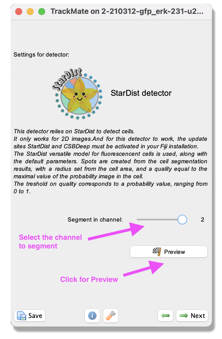
- A panel with a description of the StarDist detector opens. By clicking on the
Segment in channelslider, select the channel to segment. Here, select channel 2, which contains the DNA label. - By clicking the
Previewbutton, you can test the detector on the current frame. - When you are happy with the result, click
Next. - The detector will detect all nuclei in the selected channel for all time frames. As the movie has many time-points, this can take a few minutes.
- When the progress bar has reached the end, click
Next. - A panel to filter the detected spots according to their quality opens (more information about this filtering can be found here). In this exercise, this part can be ignored. Please click
Next.
- A panel to filter spots according to their properties (i.e. size, shape, location, or signal intensity) opens. In this exercise, do the following:
- Click the green plus sign at the bottom of the panel - a filter appears.
- Click the pull-down menu and select
Area. Here we will filter out the smallest detected objects. Make sure theAbovebutton is selected. - Drag the horizontal line (pink dashed line) to value 30.92 (approximatively). If you want to enter an exact value as threshold, just click inside the filter panel to make it active (the text becomes red) and type the number you want with key board. After 1 second it will be set as threshold.
- Click again on the green plus sign at the bottom of the panel to activate a second filter.
- Click the pull-down menu and select
Mean intensity ch2. Here we will filter out the detected objects with low intensity in Channel 2. Make sure theAbovebutton is selected. Drag the horizontal line (pink dashed line) to value 120.73. ClickNext.

- Next, a tracking panel opens. In this panel, you can select the methods for tracking objects. Here, we use the
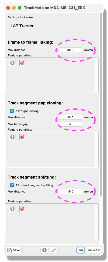
LAP trackerto account for possibly dividing cells. Please select it from the pull-down menu, and clickNext. - A panel for the LAP tracker settings opens. Int this panel, you choose how to track the cells. First, with the
Frame to Frame linkingparameter, you give the maximum distance to link two objects between frames. Here use 30 microns. Then, you can choose how many spots can be missing, and they could still be the same track. Tick theAllow gap closingbox and add values:Max distance: 30 microns andMax frame gap: 5. Next, you let TrackMate know if the tracks are allowed to split. Splitting can be caused, for example, due to cell division. Tick the boxAllow track segment splittingand insert valueMax distance: 15 microns. Below you will also see settings forTrack segment merging. Here this box should remain unticked. ClickNext.
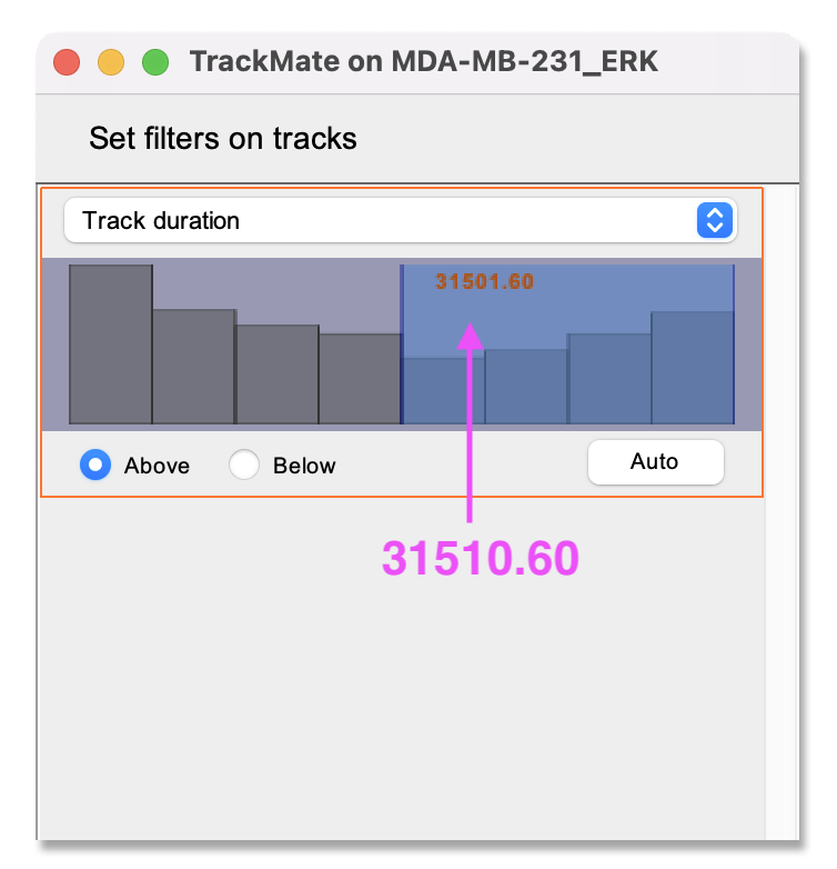
- After tracking, a track filter panel opens. In this panel, you can remove tracks according to their properties (i.e., length, speed, or location).
Here, we filter out short tracks to remove cells that migrate in or out of the field of view. As for the object filtering step described above, click the green plus sign to add a filter. Next, click on the pull-down menu and select
Track durationfrom the list. Make sure thatAboveis ticked and set the slider to about 30k. ClickNext.
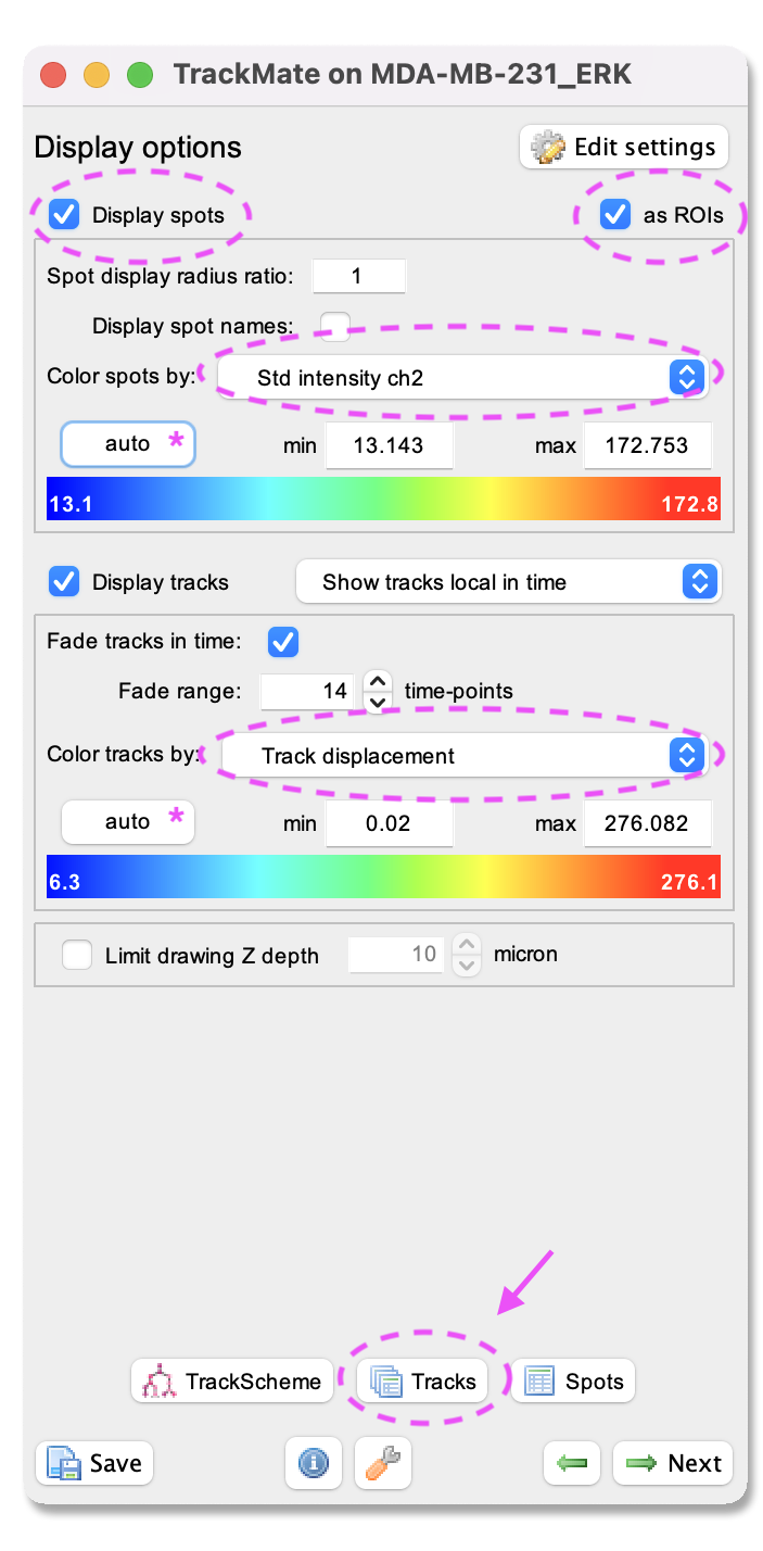
- A window with track visualization options opens. Here it is possible to edit track or object colours according to their properties.
- First, make sure that the
Display spotsandas ROIsboxes are ticked. - One option is to label the spots (nuclei) according to the standard deviation of channel 1 intensity. In this case, a blue colour will indicate that the ERK activity reporter signal is stable over time. In contrast, a red colour will show that the ERK activity reporter signal fluctuates over time. With this colouring, it is possible to visualise cells displaying ERK activity oscillations.
- To do this, select from the pulldown menu
Color spots by Mean intensity ch1. Clickautobelow to spread out the signal colour. - For the tracks, we will visualize the track displacement. First, make sure you have the
Show tracks local in timeselected from the pull-down menu afterDisplay tracks. - Next, tick the
Fade tracksin the time box and select aFade rangeof 14. Next, choose from the pull-down menu:Color tracks by Track displacement. This will show the tracks that move a short distance in blue and the longest travelled track in red. Now you can visualise if the presence of ERK oscillation corresponds to the distance travelled by the cells.
- First, make sure that the
- In this panel, you can also export the results as .CSV files. Please do so, we will need them for the analysis in MATLAB in the seconfd paty. Click on the
Tracksbutton at the bottom of the panel. A window with a lot of data shows up. Ensure you export theSpots(information about the spot) and theEdges(information about the links between 2 spots) files. Close the results window and clickNext.
- In the next panel
Plot features, it is possible to Plot some of the features of the tracks, for example, the changes of the signal intensity over time. However we cannot readily correlates the instantanous speed with the ERK intensity in nuclei, because the former is a feature of edge objects and the latter of spot objects. We will address this in a second part with a MATLAB analysis script. ClickNext. - In the next panel, there is a possibility to do different actions. For this exercise, we will export a tracking image of our experiment. From the pull-down menu, please select
Capture overlay. As you click onExecutebelow, a pop-up window opens. Here you can define the time interval you want to save. Please tick the boxHide imageand clickOK. TrackMate will generate a video of the experiment.
Track analysis with MATLAB
The zip file of the dataset contains the 2 CSV files generated from the first paty above, and a MATLAB script that reads them and investigate whether the speed correlates with ERK intensity. We outline the script here.
First let’s load the data.
clear
close
clc

% Path to the CSV files, exported from TrackMate.
spots_csv_file = 'CellMigration_WithERK-spots.csv';
edges_csv_file = 'CellMigration_WithERK-edges.csv';

%% Load CSV files into MATLAB tables.
spot_table = readtable( spots_csv_file );
edge_table = readtable( edges_csv_file );


%% Display info on tables.

fprintf( 'Header of the spot table:\n' )
head( spot_table )

fprintf( '\nHeader of the edge table:\n' )
head( edge_table )
Header of the spot table:

ans =

  8×38 table

       Var1         ID      TRACK_ID    QUALITY    POSITION_X    POSITION_Y    POSITION_Z    POSITION_T    FRAME    RADIUS    VISIBILITY    MANUAL_SPOT_COLOR    MEAN_INTENSITY_CH1    MEDIAN_INTENSITY_CH1    MIN_INTENSITY_CH1    MAX_INTENSITY_CH1    TOTAL_INTENSITY_CH1    STD_INTENSITY_CH1    MEAN_INTENSITY_CH2    MEDIAN_INTENSITY_CH2    MIN_INTENSITY_CH2    MAX_INTENSITY_CH2    TOTAL_INTENSITY_CH2    STD_INTENSITY_CH2    CONTRAST_CH1    SNR_CH1    CONTRAST_CH2    SNR_CH2    ELLIPSE_X0    ELLIPSE_Y0    ELLIPSE_MAJOR    ELLIPSE_MINOR    ELLIPSE_THETA    ELLIPSE_ASPECTRATIO     AREA     PERIMETER    CIRCULARITY    SOLIDITY
    ___________    _____    ________    _______    __________    __________    __________    __________    _____    ______    __________    _________________    __________________    ____________________    _________________    _________________    ___________________    _________________    __________________    ____________________    _________________    _________________    ___________________    _________________    ____________    _______    ____________    _______    __________    __________    _____________    _____________    _____________    ___________________    ______    _________    ___________    ________

    {'ID20994'}    20994       0        0.87727      467.92        304.57          0            42303       141     6.8714        1                NaN                 892.92                   898                   594                 1070               3.1252e+05              109.68                141.27                  144                     78                  190                    49446              21.051            -0.18132      -3.6061       -0.1431      -2.2415     0.070632       0.064366       9.3421           5.0833            0.1923             1.8378           148.33     47.735        0.81804      0.97503
    {'ID10754'}    10754       0        0.83571      451.67        218.51          0            20401        68     3.7286        1                NaN                  993.1                  1036                   482                 1167               1.0428e+05              155.98                141.02                  146                     72                  227                    14807              35.293            -0.32104       -6.021      -0.25705      -2.7649    -0.013069       -0.01824       4.2237           3.2984           -1.3372             1.2805           43.677     26.499        0.78161      0.92825
    {'ID25602'}    25602       0        0.89615      490.18        292.33          0            51303       171       7.21        1                NaN                 1040.2                  1041                   812                 1215               3.9944e+05              85.512                138.93                  144                     93                  184                    53351              19.692            -0.11814      -3.2592      -0.14992      -2.4885     0.010226      -0.010218        8.186            6.407          -0.71347             1.2777           163.31     46.657        0.94274      0.98977
    {'ID20995'}    20995       0        0.87711      482.46        273.57          0            42303       141     7.2147        1                NaN                 870.72                   888                   548                  985               3.3261e+05              78.431                139.42                  142                     85                  185                    53258              18.521             -0.1956      -5.3989      -0.13575      -2.3648     0.040536       0.073317         8.96           5.8645           -1.3124             1.5278           163.52     48.145        0.88651      0.98726
    {'ID4611' }     4611       0        0.85884      458.63         210.1          0           6000.4        20     7.6966        1                NaN                 1091.5                  1094                   843                 1413               4.8246e+05              109.33                232.76                  235                    106                  402               1.0288e+05              58.915            -0.16636      -3.9848       0.10675      0.76213    0.0078895      -0.021079        8.114           7.3583           -1.4064             1.1027            186.1     49.794        0.94321      0.98218
    {'ID7684' }     7684       0        0.83752      468.28        214.64          0            13201        44     6.1328        1                NaN                 1625.5                  1652                  1057                 1858               4.5677e+05              159.43                325.73                  308                    184                  536                    91530              87.696           -0.098066      -2.2171        0.1099      0.73554     0.075046      -0.018995       7.3124           5.2173           0.24957             1.4016           118.16     40.901        0.88759      0.97731
    {'ID29701'}    29701       0        0.87407       480.8        309.16          0            58804       196     7.4798        1                NaN                 985.05                   991                   689                 1161               4.0978e+05               106.2                135.36                  138                     89                  174                    56309              18.971            -0.11955      -2.5188      -0.18033      -3.1395     0.037025      0.0043714       8.6703           6.4975          -0.77281             1.3344           175.76     49.174        0.91339      0.98231
    {'ID15878'}    15878       0        0.83024      461.84        250.16          0            31802       106     6.7081        1                NaN                 912.99                   937                   464                 1147               3.0676e+05              114.64                147.35                  153                     83                  187                    49510              21.257            -0.21064      -4.2504     -0.094686        -1.45      0.11303     -0.0094924       8.5511           5.3345           -1.3697              1.603           141.37     45.864        0.84455       0.9781


Header of the edge table:

ans =

  8×13 table

            Var1             TRACK_ID    SPOT_SOURCE_ID    SPOT_TARGET_ID    LINK_COST    DIRECTIONAL_CHANGE_RATE      SPEED      DISPLACEMENT    EDGE_TIME    EDGE_X_LOCATION    EDGE_Y_LOCATION    EDGE_Z_LOCATION    MANUAL_EGE_COLOR
    _____________________    ________    ______________    ______________    _________    _______________________    _________    ____________    _________    _______________    _______________    _______________    ________________

    {'ID31545 → ID31681'}       0            31545             31681           2.0205            0.0037053           0.0047378       1.4214         62254          496.72             311.66                0                 NaN
    {'ID19256 → ID19400'}       0            19256             19400            10.28             0.010471            0.010687       3.2063         38853          487.15             248.62                0                 NaN
    {'ID14361 → ID14477'}       0            14361             14477           5.4277             0.010471           0.0077653       2.3297         28652          462.22             245.67                0                 NaN
    {'ID17824 → ID18039'}       0            17824             18039           1.2679             0.010471           0.0037531        1.126         36152          489.52             240.16                0                 NaN
    {'ID17160 → ID17216'}       0            17160             17216           83.774             0.010471            0.030507       9.1528         34652          461.37             257.23                0                 NaN
    {'ID7684 → ID7827'  }       0             7684              7827          0.75557             0.009246           0.0028973      0.86923         13351          468.56             214.31                0                 NaN
    {'ID10506 → ID10604'}       0            10506             10604           3.6989             0.010471           0.0064104       1.9233         19951          452.52             219.05                0                 NaN
    {'ID22343 → ID22544'}       0            22343             22544           84.232            0.0017781            0.030591       9.1778         45153          487.83             277.45                0                 NaN
As said above, we need to correlate a value that belongs in two different tables: the mean ERK intensity in the spot table, and the speed in the edge table.
The speed is defined as an edge feature, because you need two spots to define a displacement and a time interval, hence a speed.
But we want to plot the speed and intensity for the same spot.
The trick is to use the spot ID value, which is unique in a tracking session.
The edge table has two columns that store the ID of the 2 spots it links: SPOT_SOURCE_ID and SPOT_TARGET_ID.
So we need to join the 2 tables, using the ID column in the spot table and (for instance) the SPOT_TARGET_ID in the edge table.
In MATLAB, this is done as follow:
T = join( edge_table, spot_table, ...
    'LeftKeys', 'SPOT_TARGET_ID', 'RightKeys', 'ID', ...
    'LeftVariables','SPEED' , 'RightVariables', 'MEAN_INTENSITY_CH1');
head(T)
ans =

  8×2 table

      SPEED      MEAN_INTENSITY_CH1
    _________    __________________

    0.0047378          917.44
     0.010687          787.33
    0.0077653          862.49
    0.0037531          907.65
     0.030507          1016.8
    0.0028973          1606.6
    0.0064104          1060.7
     0.030591          1063.9
And finally we can visualize whether we have some correlation with a scatter plot.
figure
scatter( T.SPEED, T.MEAN_INTENSITY_CH1, 'k.' )
xlabel( 'Speed (µm/sec)' )
ylabel( 'ERK nuclei intensity' )
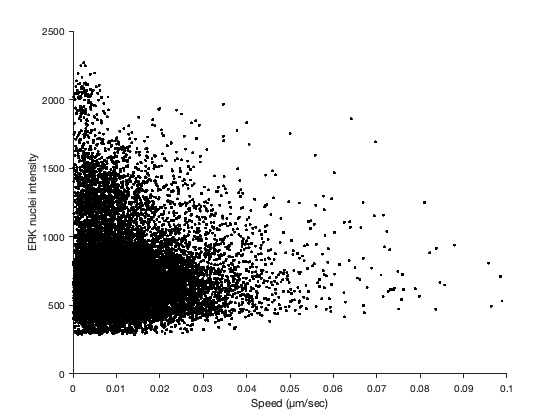
It’s rather unclear with that many points. Let’s try to plot the density of points.
figure
histogram2( T.SPEED, T.MEAN_INTENSITY_CH1, 'FaceColor', 'flat' )
view( 2 )
grid off
box off
xlabel( 'Speed (µm/sec)' )
ylabel( 'ERK nuclei intensity' )
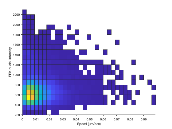
It’s not more clearer. Let’s analyze the correlation coefficient.
[ R, P ] = corrcoef( T.SPEED, T.MEAN_INTENSITY_CH1 );

fprintf( 'Correlation coefficient: %.2e\n', R( 1, 2 ) )
fprintf( 'P-value for the correlation: %.2f\n', P( 1, 2 ) )
Correlation coefficient: 4.00e-03
P-value for the correlation: 0.56
We have to conclude that this dataset does not show a correlation between instantaneous speed and ERK intensity in the nucleus. Maybe we need to filter out some spots with low speed, or investigate tracks as a whole. But this is left as an exercise to the reader.
Tracking T-cells imaged in bright-field with a custom model in the StarDist detector
You can also use a custom model, that you have trained yourself and packaged as a zip file. We recommend using the dedicated notebooks on the ZeroCostDL4Mic platform to do so. Check the ZCDL4M wiki page dedicated to training StarDist to generate such a model.
In this tutorial we will track T cells imaged in bright-field with a model we trained ourselves. You can find the image and the model (packaged as a zip file) on Zenodo:
![]()
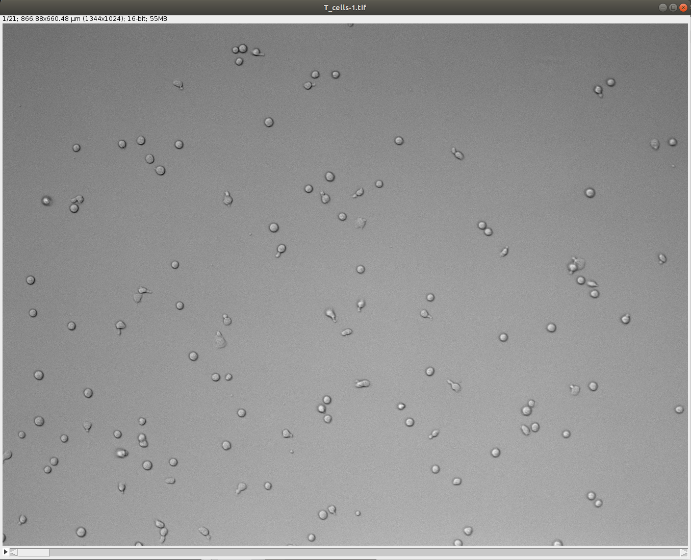
First open the tutorial image called TCellsMigration.tif in Fiji provided in the tutorial data.
Launch TrackMate. In the second panel titled Select a detector, choose StarDist detector custom model and click Next. Its configuration panel requires several parameters:
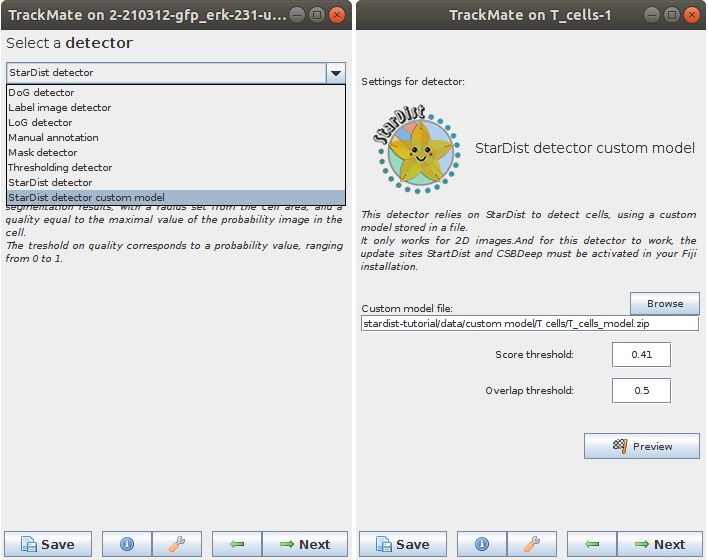
- In the Custom model file text field, you need to enter the path to a StarDist model packaged as a zip file (or use the Browse button to navigate to the folder). In the tutorial dataset the file is called
StarDistModel-TCellsBF.zip. - Score threshold correspond to the threshold on the probability map to identify object. It accepts values from 0 to 1.
-
Overlap threshold correspond to the threshold used in non-maxima suppression step used to separate touching/overlapping objects; it accepts values from 0 to 1.
-
Set these parameters and click Preview button to test the detector on the current frame. Here is an example of what we get on the first time-point of the tutorial image (using default parameters):
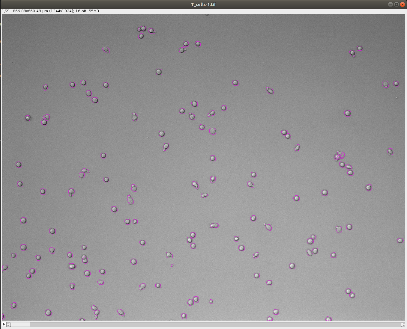
-
In case the results are satisfying, click Next to perform detection in the full time-series. After the detection is finished, continue with the following steps same as in standard TrackMate workflow. Using the default tracker (Simple LAP tracker) with the default parameters we get this result:
Generation of 3D labels by tracking 2D labels using TrackMate
In this tutorial, you will learn how to generate 3D labels using TrackMate. The segmentation of 3D objects can be very hard. Deep Learning proves to be very efficient but there are still many models and algorithms that only work for the 2D case. In this tutorial, we “hack” TrackMate to segment 3D objects using the 2D StarDist segmentation algorithm. We trick TrackMate into thinking a 3D image is a 2D movie over time. We track the fake 2D objects in Z, and use the resulting track information to rebuild the 3D segmentation of objects. The following step-by-step tutorial shows how to do this.
First download the dataset from Zenodo:
![]()
The dataset onctains the raw data but also the intermediate label images in case you want to play with them directly.
- Open Fiji.
- Open the
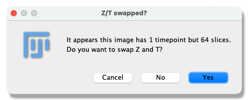
Spheroid-3D.tifimage in Fiji. This image is a Z stack of MCF10DCIS.com 3D spheroids that have been stained with DAPI to visualise their nuclei. - Open TrackMate Plugins › Tracking › TrackMate. As the image is a 3D Z stack, TrackMate will ask you to swap the Z and T dimensions. This is what we want; click
Yes.
- The start panel will open, showing information about the image dimensions. Click
Next. - The
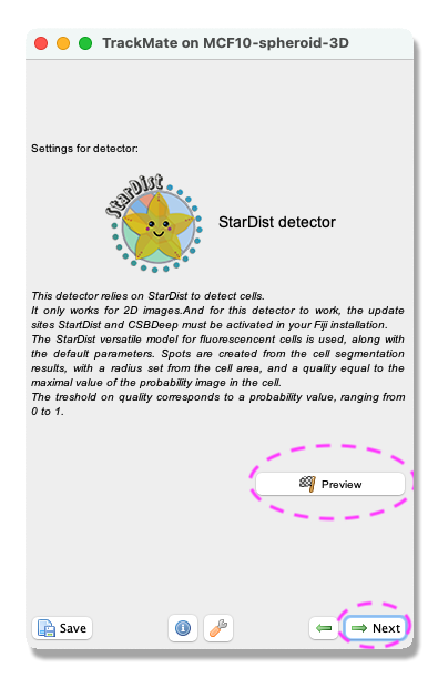
Select a detectorpanel opens. From the pull-down menu select theStarDist detector. ClickNext. - A panel with a description of the StarDist detector opens. By clicking the
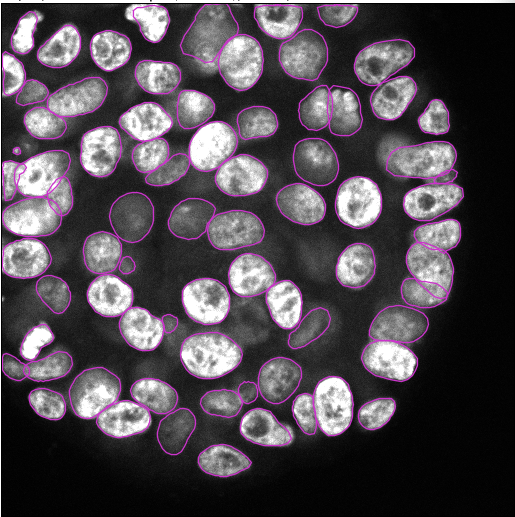
Previewbutton, you can test the StarDist detector on the current frame. When you are happy with the result, clickNext.
- The detector will detect all nuclei in the selected channel for all time frames. This can take a few minutes.
- When the progress bar has reached the end, click
Next. -
A panel to filter the detected spots according to their quality opens (more information about this filtering can be found here). In this exercise, this part can be ignored. Click
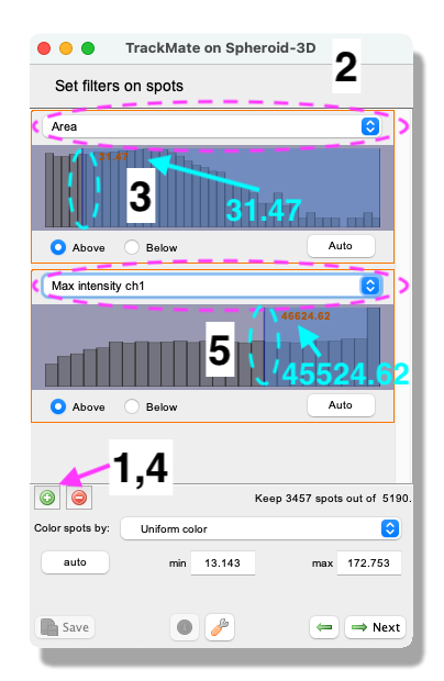
Next. - A panel to filter spots according to their properties (i.e. size, shape, location, or signal intensity) opens. In this exercise, do the following:
- Click on the green plus sign at the bottom of the panel - a filter appears at the top of the panel.
- Click on the pull-down menu and select
Area. Here we will filter out the smallest detected objects. Make sure theAbovebutton is selected. - Drag the horizontal line (cyan dashed line) to value 31.47.
- Click on the green plus sign at the bottom of the panel again - a new filter appears.
- Click on the pull-down menu and select
Max intensity ch1. Here we will filter out the objects that have low intensity. Make sure theAbovebutton is selected. Drag the horizontal line (cyan dashed line) to value 45524.62. - Click on
Next.
- Next, a tracking panel opens. In this panel, you can select the methods for tracking objects. Here, we use the
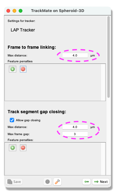
LAP tracker. Please select it from the pull-down menu, and clickNext. - A panel to choose the LAP tracker settings opens. With this panel, you choose how to track the cells. First, with the
Frame to Frame linkingparameter, you give the maximum distance to link two objects between frames. Here use 4 microns. Next, you tell Trackmate how many spots can be missing and still be the same track. Tick theAllow gap closingbox and add values:Max distance: 4 microns andMax frame gap: 3. ClickNext.
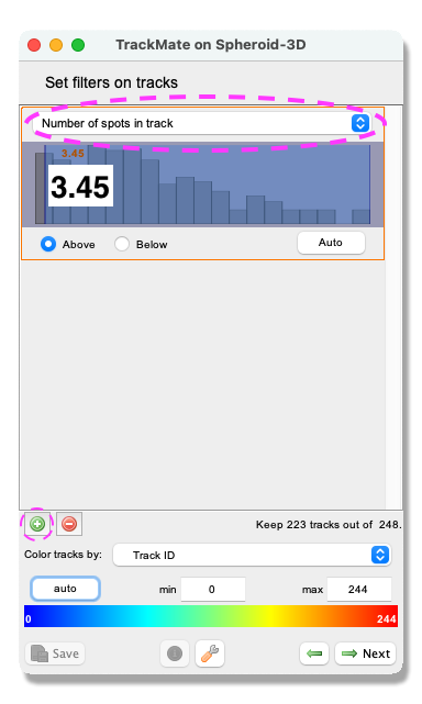
- A Track filter panel opens. In this panel, you can remove tracks according to their properties (i.e., length, speed, or location). Here, we filter out the shortest tracks to remove possible artefacts. Similarly, as in the object filtering above, click the green plus sign to add a filter. Click the pull-down menu and select
Track durationfrom the list. Make sure that theAboveoption is ticked and set the slider to 3.45. ClickNext.
- A window with track visualization options opens. Here it is possible to edit track or object colours according to their properties. We don’t need to use it in this exercise. Click on
Next. - Click on Next again.
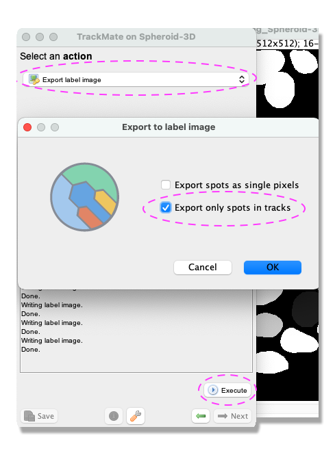
- You should have reached the
Select an actionpanel. In this panel, there is a possibility to do different actions. For this exercise, we will export a label image of the tracked objects. From the pull-down menu, selectExport label imageand click onExecute. - From the pop-up window, tick the box
Export only spots in tracksto eliminate any object not linked to a track and clickOK.
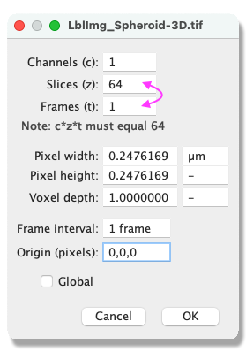
- The label image is now exported. Remember to change the dimensions back from T to Z in Fiji Image › Properties and to save your image File › Save as….
- The label image can be viewed in 3D for instance using FPBioimage, and further analysed using the 3D ImageJ Suite.
Citations
If you use this detector for your research, please be so kind as to cite the StarDist and the TrackMate papers:
doi:10.1007/978-3-030-00934-2_30
Dmitry Ershov, Joanna W. Pylvänäinen, Jean-Yves Tinevez - July 2021