The content of this page has not been vetted since shifting away from MediaWiki. If you’d like to help, check out the how to help guide!
Overview of ‘Xlib’
A set of prospective ImageJ plugins is maintained by the group for 3D-Microscopy, Analysis and Modeling of the Laboratory for Concrete and Construction Chemistry at Empa Dübendorf, Switzerland. The plugins include automated imaging tools for filtering, data reconstruction, quantitative data evaluation and data import, as well as tools for interactive segmentation, visualization and management of image data.
Since the research focus of our group is on 3D imaging, all of our plugins are able to deal with either 2D or 3D image data. 3D image data is always represented by image stacks. 3D processing may include slice-wise 2D processing of all images in the stack or, sometimes more important, true 3D processing.
Each one of the new plugins includes a help button where basic remarks about the functionality and a description of the parameters is provided. This feature does not correspond with the ImageJ philosophy assuming the help documentation to be available on the internet only. However, we consider the help button as a handy feature.
The user might be surprised to realize that some of the tools are apparently already existing in other plugins of ImageJ or Fiji. Those tools are for instance “FFT 2D 3D”, “Image Calculator”, “Distance Transform”, “Transform 2D 3D” and others. The reason for this apparent redundancy is that the original tools incorporate major restrictions which are elimintated in the new plugins. Each one of the available tools and its advantage is shortly being presented below.
The following plugins are included:
Data Analysis:
- “Closest Cluster”: Engine for finding the closest candidate to a list of chemical substances
- “Import DMP”: Import elementary image data from “.dmp” files (e.g. originating from MATLAB)
Filtering:
- “Anisotropic Diffusion”: Anisotropic diffusion
- “Canny Edge”: Canny edge detection
- “Cluster Image”: Clustering of images
- “Disconnect Particles”: Particle disconnection
- “Distance Transform”: Distance transform
- “FFT 2D 3D”: Fast Fourier transform of arbitrary sized images
- “Image Calculator”: Utterly generalized image calculator
- “Labeling 2D 3D”: Labeling of disconnected binary mask objects
- “Median 2D 3D”: Conventional and multidimensional median filtering
- “Remove Background”: Remove background from image by polynomial approximation
- “Roundness 2D 3D”: Roundness filter
- “Skeletonization 2D 3D”: Skeletonization of binary masks
- “Stripe Filter”: Removal of horizontal and vertical stripes
- “Transform 2D 3D”: Generalized image transforms
- “Wavelets 2D”: Wavelet decomposition and reconstruction
Reconstruction:
- “Filtered Backprojection”: Filtered backprojection of projections
- “Projections Sinograms”: Conversion of sets of projections into sinograms and vice versa
- “Reconstruct 3D from 2D”: Reconstruct virtual 3D structures from given 2D structures
Evaluation:
- “Particle Size Distribution”: Calculate particle size distribution of binary particle structures
- “Phase Image Evaluation”: Evaluate images consisting of a number of homogeneous phases
- “Pore Size Distribution”: Calculate pore size distribution of binary pore structures
Editors and Viewers:
- “Display Volume”: Interactively visualize 3D volume by an orthogonal slicer
- “Edit Label Region”: Engine for interactive editing of labeled binary 2D or 3D particle structures
- “Segment Phases 3D”: Engine for basic interactive segmentation of images and volumes
- “View 3D Mask”: Rendering of 3D image masks
Data Analysis
Plugins of this section offer importing, handling or analysis of special data formats that are unknown to ImageJ, but interesting for special purposes.
Closest Cluster
This plugin provides an engine for finding the most probable chemical compositions of some given energy dispersive spectroscopy (EDS) data. From a set of proposed chemical formula, a ranking of the probability of matching with the candidate EDS data is calculated.
A step by step tutorial for the clustering and phase identification of EDS maps is provided in the manual entitled “Instructions for the Phase Clustering and Identification Using the Plugins for ImageJ”.
The program can be used in combination with the “Cluster Image” plugin. Thereby for a resulting set of cluster centers, the program provides the most probable cluster membership.
Import DMP
DMP is a simple data format for the storage of 2D images. It is used at IBT from the ETH and University of Zürich. The first two short integer entries of the data file are reserved for providing the width and the heigth of the image. The next short integer is reserved. Thereafter (i.e. after the first 6 bytes) follows the image data itself, each pixel given by a 32-bit floating number.
A short MATLAB code for writing such an image variable “image” with the size “width” and “heigth” is given below:
fid=fopen(file,'w');
fwrite(fid,size(image,2),'uint16');
fwrite(fid,size(image,1),'uint16');
fwrite(fid,0,'uint16');
fwrite(fid,image','float32');
fclose(fid);
Reading the a DMP image with MATLAB can be achieved like this:
fid=fopen(filename);
dim=fread(fid,3,'uint16');
width=dim(1);
height=dim(2);
data=zeros(height,width);
for ii=1:height
    data(:,ii)=fread(fid,width,'float32');
end
fclose(fid);
Filtering
The filtering functions accept one or more images or stacks of images where some filtering techniques are applied to. Generally, the following filtering functions work on 2D images, slice-wise 2D, as well as in true 3D mode if it is applied to image stacks.
Anisotropic Diffusion
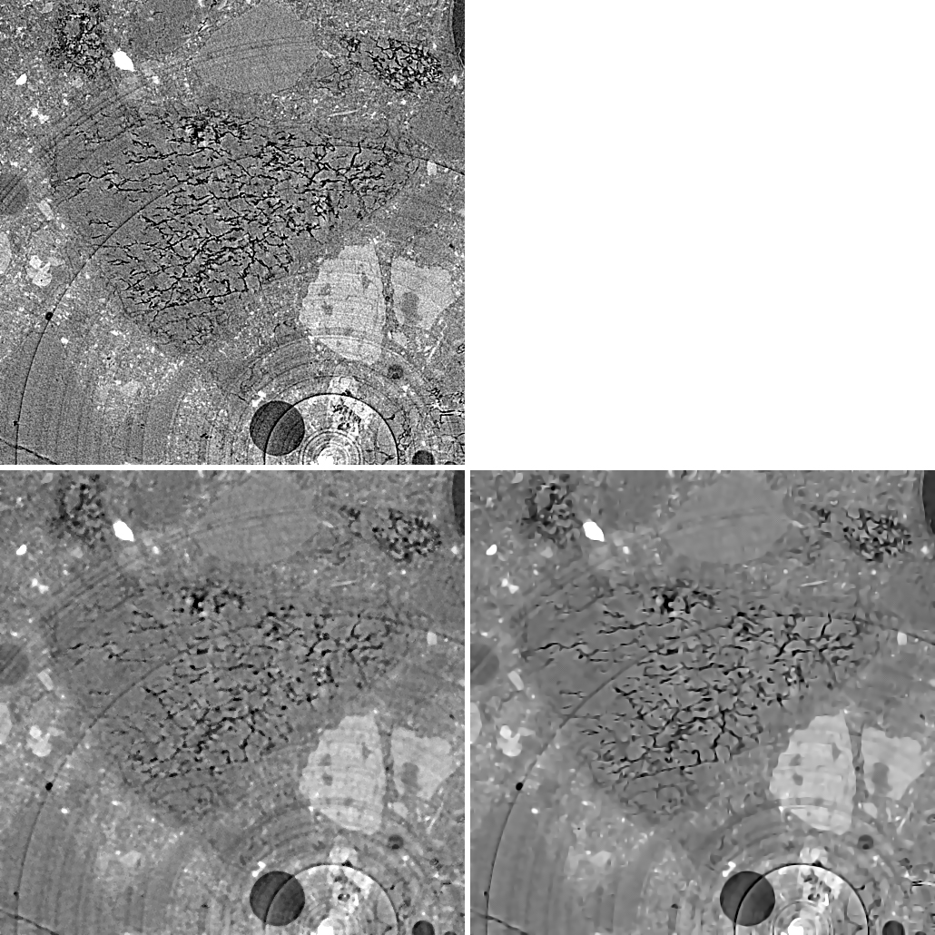
CT slice after strong alcali aggregate reactions (top) and edge preserving / smoothing filtering with a 4x4 median (bottom left) and anisotropic diffusion (bottom right).
The mechanism of heat diffusion has been used as the basics for image filtering. Thereby, the image values are understood as temperature values and image blurring represents the process of heat transport blurring. The key idea is the introduction of anisotropy, i.e. of diffusion characteristics that are depending on the pixel environment and the transfer direction. The local anisotropy is assigned according to the direction and magnitude of the image gradient, introducing high diffusion rates at low gradients and low diffusion rates at high gradients. Hence, the anisotropic diffusion characteristics are defined according to an ellipse in 2D or an ellipsoid in 3D perpendicular to the gradient vector.
The corresponding partial differential equation had first been numerically approached in 1990 by a fast algorithm of Perona and Malik [Perona1990] by defining the elliptic diffusion shapes by means of simple box filtering. Way better results can be obtained with the technique of Tschumperlé and Deriche [Tschmperlé2005] from 2005 by setting the tensor field according to the Eigenvalues and Eigenvectors in order to drive the diffusion. As expected, this approach is however more time consuming.
The filter is a brilliant edge preserving / smoothing filter for intelligent noise reduction. In particular, the implementation of Tschumperlé and Deriche outperforms other approaches in respect of the distinction between coherent edges and noise. The figure above shows a comparison between anisotropic diffusion (bottom right) and median filtering (bottom left) of a CT slice from concrete after strong alcali aggregate reactions (top). Anisotropic diffusion filtering is outstanding by better preserving the cracks while flattening inhomogeneities due to noise (please note center regions).
The filter works in 2D as well as in 3D.
Canny Edge
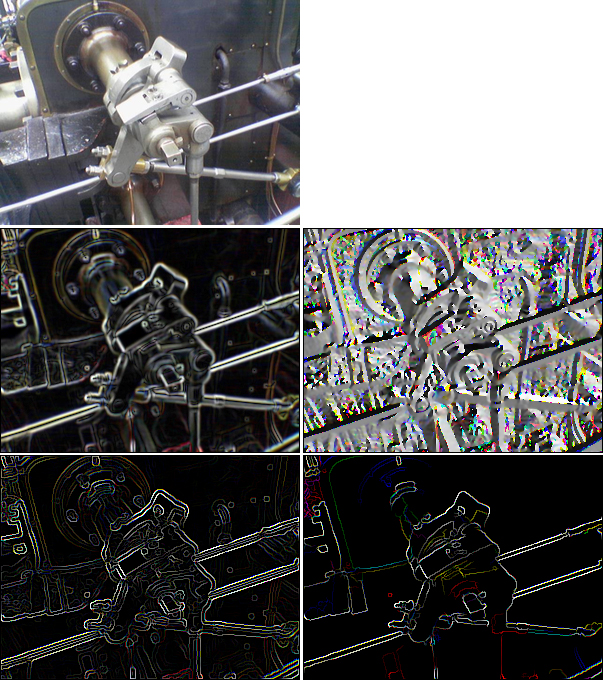
Valve image (left) and the results from the Canny filter. Top: original image, 2nd row: magnitudes of gradient vectors, angles of gradient vectors, 3rd row: magnitudes after non-maxima suppression, and the connected regions after double thresholding the maximal magnitudes.
In 1986, J. Canny has proposed an excellent edge detection filter [Canny1986] that due to its performance became famous. The filter is based on a fast numeric approach for the calculation of the direction-dependent first derivative, i.e. the gradient vector function of an image. The Canny filter is well known for 2D imaging, yet it is barely supported in 3D. This plugin supports both, the 2D and the 3D implementation. It additionally supports preceding Gauss filtering, optional non-maxima suppression for the extraction of the edges, as well as a function for double thresholding and joining the connected regions. Double thresholding means that an upper threshold is used for extracting the relevant edges, while a lower threshold is provided for adding residing connections between the extracted edges. The plugin returns the magnitudes and the angles of the gradient vector functions.
The results of a Canny filtered image of a valve image is shown in the upper figure (top: original image). The gradient magnitude and angles are presented (2nd row), as well as the magnitudes after non-maxima suppression and also after joining the connected regions (3rd row).
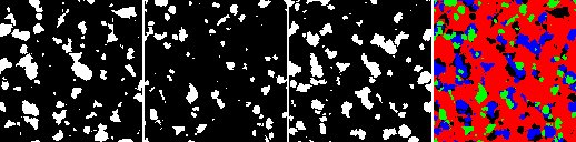
Cluster Image
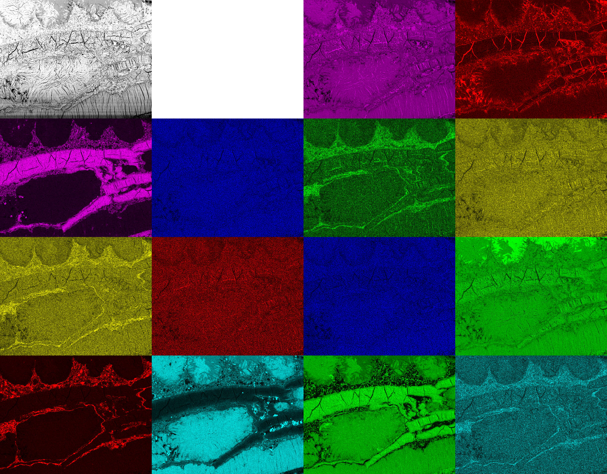
Image acquired by BSE and EDX maps at the same local position showing the amounts of Ca, C (1st row), Al, Cl, Fe, K (2nd row), Mg, Mn, Na, O (3rd row), P, Si, S, Ti (4th row).
Cluster analysis is a technique of statistical data analysis for grouping sets of objects. It is used in machine learning, data mining, pattern recognition, information retrieval, bio-informatics and can also be applied to image analysis. Different clustering definitions and algorithms have been proposed using connectivity, distance to the cluster center, statistical distribution, or density rates as optimization parameters for building clusters.
In image analysis, mainly two algorithms are prominent: the k-means algorithm and the mean shift algorithm. They have been implemented together with a third one, fuzzy c-means clustering.
The k-means algorithm [Kanungo2002] minimizes the square sum of the distances of each data point to its assigned cluster center. It starts with a random association of the data points to an initially determined number of clusters. Using an iterative optimization procedure it converges quickly to stable data assignments to clusters. K-means clustering is popular because it is very fast.
The mean shift clustering method [Funkunaga1975] optimizes the cluster centers such that the data densities within the clusters which are maximized. Within kernels of a given size around each data point, the centroid of all points inside of the kernel is determined and the sphere shifted accordingly. After iterative repetition of this process, the sphere remains stationary. The data point is then assigned to this final cluster center. The algorithm can be understood as like the walk to the closest peak in a mountain landscape. Within a certain perimeter, the highest target is being located and reached. From thereon, the next target within the same perimeter is located and reached again. This process is iteratively carried on until the top within the selected perimeter is reached. Depending on the perimeter size, different hills or sub-hills will be achieved. If the perimeter is larger than 400km, you will reach the Mont Blanc from anywhere in Switzerland. If it is larger than 20’000km, the Mount Everest will be reached from any point in the world. If its size is only a some meters, you will probably end up on the top of a building.
Fuzzy c-means clustering [Bezdek1984] allows a data point to be assigned to more than one clusters. The affiliation to a cluster is given by a membership value ranging from zero to one. The sum of all memberships for a data point is unity. Hence, the assignment of a data point to a class is not unequivocal but relative. The degree of belonging to a class is related inversely to the distance from the data point to the cluster. It also depends on a parameter that controls how much weight is given to the winning cluster. With fuzzy c-means, the centroid of a cluster is the mean of all points, weighted by their degree of belonging to the cluster. The finally winning class is the one with the highest ranking. The process of the fuzzy c-means algorithm is very similar to the k-means algorithm.
Expectation-maximization (EM) clustering [Dempster1977] iteratively finds the maximum likelyhood estimation of a Gaussian distribution fit of the original N-dimensional distribution of pixel values. The EM iteration alternates between performing an expectation (E) step, which creates a function for the expectation of the log-likelihood evaluated using the current estimate for the parameters, and a maximization (M) step, which computes parameters maximizing the expected log-likelihood found on the E step.
The plugin also allows clustering by using ELKI (Environment for Developing KDD-Applications Supported by Index-Structures, developed by the ELKI team). ELKI is an open source data mining software written in Java. In addition to multiple features, ELKI offers various ways for clustering. An ELKI wrapper for the clustering of images is included with the Image Clustering plugin. When the respective elki.jar bundle is placed in the ImageJ plugins directory, image clustering with ELKI is possible. The required specification parameters for the ELKI clustering algorithm together with its parameters can be defined by the user.
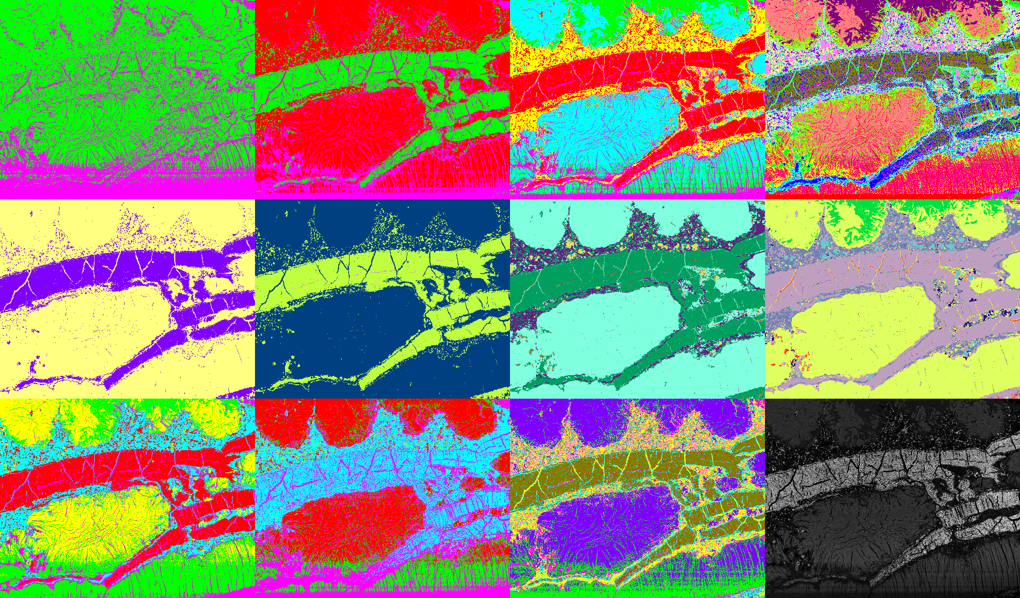
Results from clustering of the 15-dimensional image data space displayed in the figure above. First row: k-means for 2 (left), 3, 5 and 16 (right) clusters. Second row: mean shift for the seeking perimeters 100 (left), 70, 60 and 50 (right). Third row: fuzzy c-means clustering for 5 clusters at fuzziness 1.1 (left) and 4.0, 16 clusters at fuzziness 2.0, and its fuzziness membership values (right).
As an example, ESEM images of a natural cement analogue (Maqarin, Jordania) is provided in the figure to the upper right. A backscatter electron microscope (BSE) image (top left) and image maps acquired from energy-dispersive X-ray spectroscopy (EDX) at the same location forked into 14 different elements (see figure above) are used as the basis for clustering. Thus together with the BSE image, the clustering is achieved from a 15-dimensional vector space. In the figure below, some results from different clustering algorithms and parameter settings are displayed. The first row shows results from the k-means, the second one from the mean shift, and the third one from fuzzy c-means clustering. K-means clustering (1st row) requires the number of clusters as an input parameter. The results for 2 (left), 3, 5 and 16 (right) clusters are provided. Slightly different results provides mean shift clustering (2nd row) which requires the size of the seeking perimeter as input parameter. It is determined at 100 (left), 70, 60 and at 50 (right). Fuzzy c-means clustering (3rd row) requires the number of clusters and the fuzziness as input parameters. The results are displayed for 5 clusters at fuzziness 1.1 (left) and 4.0, for 16 clusters at fuzziness 2.0, as well as an image showing its fuzziness membership to the cluster with the highest respective ranking at each location (right).
Clustering can also be applied to one dimensional spaces (i.e. from a single gray level image), or for color images where the R, G, B color channels provide a 3-dimensional vector space. Clustering thus provides an elegant way for automatic segmentation of 2D images or 3D image volumes containing different phases.
Disconnect Particles
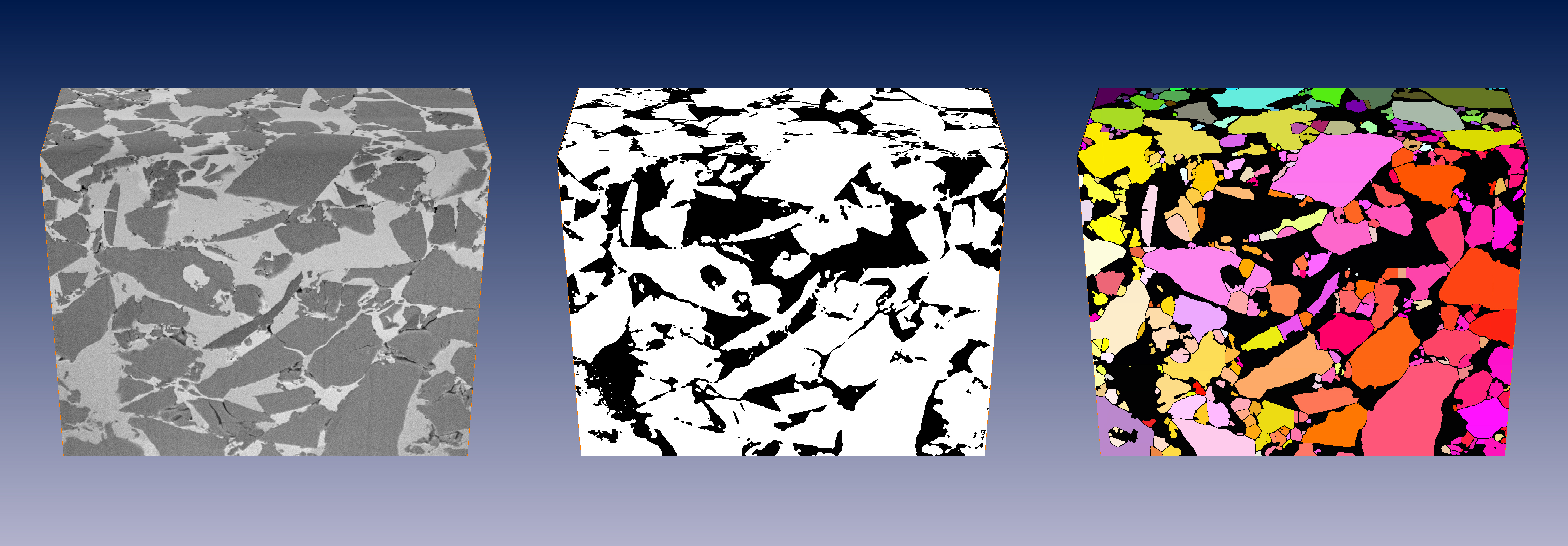
3D FIB-nanotomography of cement grains (left), subsequent thresholding (center), disconnected (k=0.7) and labeled particles (right).
In particle analysis from imaging due to the resolution limits, the particles might be wrongly connected at various locations if they are located too close to each other. To remedy such connections, an algorithm for disconnecting them at their bottle necks has been implemented [Münch2006]. If requires a parameter k ranking from [0…1] controlling the disconnection. At k=1, particle separation occurs at any bottle necks while at k=0, no separation at all is being performed. The optimum depends on the data and is usually somewhere around k=0.7 inducing marked bottle necks to be carved and small bottle necks to be left unchanged.
Results from cement grains acquired by 3D FIB-nanotomography are displayed in the figure above. To the left, the original data volume is visualized. The center image shows the mask after image thresholding. Particles close to each other are erroneously interconnected at various locations. The image to the right shows the volume disconnected at k=0.7 and labeled subsequently.
Distance Transform
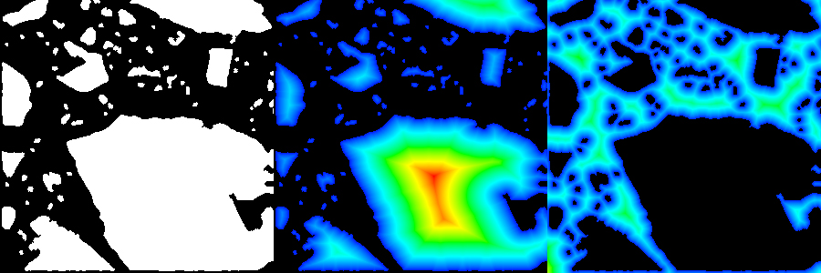
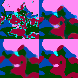
Binary mask from cement particles (left) and Euclidian distance transform of it (center) and of its reversed mask (right).
Fast distance transform of image masks is useful for many morphological imaging applications. In an age of increasing data size, processing speed is of ultimate priority. A modern approach [Saito1994,Meijster2000] allows the generation of the distance transform even in linear time. The implementation in this plugin allows the calculation of Euclidian, Chessboard, or Citymap distance transform in both, 2D and 3D.
Mask containing 3 black dots only (left) and its Euclidian, Chessboard and Citymap (right) distance transform.
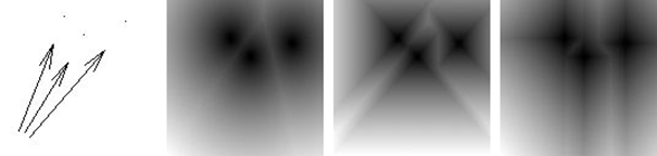
FIB-nt image (427x768 pixels) from cement paste (left) and the magnitudes (center) and angles (right) of its Fourier transform.
In the upper figure, a binary mask from cement particles (left) is processed by using the Euclidian distance transform (center). The transform of the inverse mask is also given (right). The distances are visualized by using a color lookup table from blue (low values) to red (high values). The effect of different distance metrics is displayed in the lower figure. A simple mask consisting of 3 single black dots is provided (left). Next to it, the results of the Euclidian, Chessboard and Citymap (right) distance transform is shown.
FFT 2D 3D
The fast, well known and widely used Cooley-Tukey radix-2 algorithm for the calculation of the discrete fast Fourier transform (FFT) only works on data whose size is equal to a power of two. In order to provide FFT on data of different size, the data is usually extended to the next higher power of two. In many cases, this approach is sufficient, in particular if the periodical nature of the transformed data function is not relevant. However, if the period length is important and must be left unchanged, FFT on the original data size is required. This can be achieved by using the Bluestein algorithm [Bluestein1968,Rabiner1969]. Since to our best knowledge, there is no ImageJ plugin available that permits FFT for non-radix-2 sized periods, this plugin has been built. It correctly calculates the complex FFT on 2D and 3D images of arbitrary size. It optionally provides the real and the imaginary part, or the magnitude and the angle images. Moreover, it allows a logarithmic or square-root based scaling to be introduced in order to lower the contrast among the FFT coefficients. This feature is useful if the FFT function is used for display purpose. The reversibility of the FFT transform is supported for all these options.
The figure to the right shows a sample FIB-nt image from cement paste (left) with a width of 427 and a height of 768 pixels. The magnitudes and angles of its Fourier transform is scaled by a logarithmic funcion for improving the visibility of the small coefficients. The inverse FFT transform of the center and right images reconstructs the original function (left) again without any loss of precision.
Image Calculator
Many image calculators allowing various arithmetic operations are already implemented in ImageJ, including the “Image Calculator”, the “Calculator Plus” as well as the entire list of functions in “math”, all of them under “Process”. So why “yet another image calculator”, you might ask. The reason is that our image calculator is easily able to perform the possible tasks of all of the above listed plugins and much more. The conceptual idea is to provide a list of all the images and image stacks that are currently opened in ImageJ and assign them to symbolic names (i0, i1, i2,…). In a text field, the user can then provide his own code he wants to be applied to the images. The image calculator is working for both, single 2D images and for 3D image volumes.
The input images (or 3D image stacks) are named to ‘i0’, ‘i1’, ‘i2’,… in the order they have been loaded to ImageJ. Using these variables, any java-operations yielding values (i.e. basic operations or calls to java-functions) can be executed.
The image calculator has two different operation modes. The first mode (see first few examples) just returns just a single value calculated from one or more input images. This operation is then assigned to each single pixel or voxel. The second mode (see last few examples) accepts multi-line coding using any type of java-syntax. It requires an output image (or volume) being defined, calculated, and finally being returned by using the statement like “return new Object[] { mm, out };”, the variable ‘mm’ holding an integer array containing the image (or volume) size in pixels (or voxels) in x, y (and eventually z); the variable ‘out’ holding the image (volume) data itself.
In the following, some examples are presented:
left: image i0, 2nd: image i1, 3nd: image i2, right: mean value of the images i0, i1 and i2
(i0 + i1 + i2) / 3
Make sure there are three images loaded on ImageJ such that i0, i1, and i2 are the ones to be processed. Subsequently, the above command will return an image providing the mean value of images i0, i1 and i2 (see rightmost image to the right).
The following command makes use of java-internal classes. Since global import statements of many useful classes are usually not defined per default, the full path to the java library (here: “java.awt.Color”) should be provided.
left: image i0, right: mask where regions higher than 170 are colored in red
(i0 > 170)?
	java.awt.Color.red.getRGB() : java.awt.Color.black.getRGB()
displays a mask where values higher than 170 are set to a red color, while the remaining are set to black. Like in the the previous example, it is important to set the argument “Format for output image” to “int color” in order to enable color output.
The following operation makes use of plain integer values for the color definition.
left: image i0, 2nd: image i1, 3rd: image i2, right: colored mask out of images i0, i1, i2
The value “-16777216” represents black, the value “-65536” red, the value “-16711936” green, the value “-16776961” blue color.
(i0==255)? -16711936 :
	((i1==255)? -16776961 : ((i2==255)? -16777216 : -65536))
takes three binary images i0, i1, i2 and creates a colored mask out of it (see rightmost image to the right). Like in the the previous example, this operation requires setting the argument “Format for output image” to “int color”.
left: image i0, right: power of two of image i0
The operation
Math.pow(i0, 2.)
yields the power of two of the image i0. It is recommended to set the value of “Format for output image” to “float gray” (or at least “short gray”, instead of “byte gray”) in order to avoid exceeding the value range. If “byte gray” is selected, pixel values larger than 255 are set to 255.
left: i0, right: copy of image i0 overlayed by a ramp
The operation
i0 + x
will calculate a copy of the image i0 overlayed by a horizontal ramp. The value of ‘x’ (and ‘y’, and ‘z’ for 3D volumes) is internally defined as the local x-coordinate (y-coordinate, and z-coordinate for 3D volumes).
left: image i0, right: ramp with the same size as image i0
The code line
x // i0
creates the ramp only.
In this case, instead of an image operation, just the value of “x” (which would create no image itself) is returned. A commented out “i0” is attached to the command. The reason why this is necessary is to provide a clue about the size of the resulting image which now turns out to be equal to the size of image i0. Hence, the content of the image i0 is actually not being used, it serves as a template for the resulting size only.
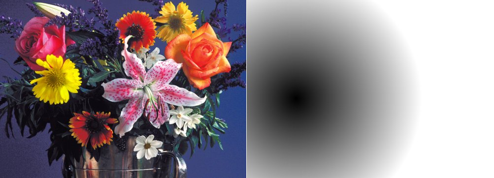
left: image i0 defining image size, right: halo centered at (100, 200)
The following code
Math.sqrt(Math.pow(100 - x, 2) + Math.pow(200 - y, 2)) // i0
calculates an image of the same size as image i0, but containing only a halo centered at (100, 200). Since the code for the generation of the image does not contain neither operations on input images, nor any definitions for the image size, the parser searches for other hints for determining the output image size and takes the reference to ‘i0’ even though it is commented out.
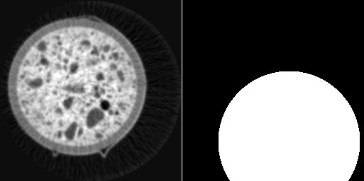
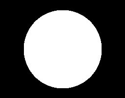
left: image i0, right: circular mask around (100, 200)
The following command line
(Math.sqrt(Math.pow(150 - x, 2) +
 Math.pow(200 - y, 2)) < 100)? 255 : 0 // i0
creates an image containing a circular mask around point (100, 200).
As in the previous example, the comment “// i0” is required for defining the size of the new image according to the size of i0.
left: image i0, right: binary thresholding of i0 by value 128
The following command line
(i0 >= 128)? 255 : 0
creates a binary image mask by thresholding the image i0 with a threshold value of 128. Please note that single-row assignments as shown in all previous examples always need to return a pixel value. That’s the reason why ‘if’-statements are not possible in this context and must be bypassed by a ‘?’ operation.
left: image i3, right: content of image i3 inside of a circle
The following code
(Math.sqrt(Math.pow(mx / 2 - x, 2) +
 Math.pow(my / 2 - y, 2)) < mx / 2)? i0 : 0
takes the content of the image inside of a circle only and removes the regions outside. Please note: this code fragment makes use of the predefined variables ‘mx’ and ‘my’ holding the image size in x and y. For image stacks, the variable ‘mz’ is defined as well.
left: image i0, center: image i1, right: exclusive OR of images i0 and i1
Finally,
(((int)i0 ^ (int)i1) > 0)? 255 : 0
performs an exclusive OR operation of image i0 and image i1.
The above examples show that any pixel- or voxel-wise operation can be provided in a single command line as soon as it follows the Java notation. The plugin is however able to do much more. Instead of pixelwise operation mode, image-wide Java code fragments can be provided. For example,
float[] out = new float[i0.length];
for (int ii = 0; ii < out.length; ii++)
	out[ii] = (i0[ii] + i1[ii] + i2[ii]) / 3f;
return new Object[] { m0, out };
performs the same operation as the pixelwise operation (i0 + i1 + i2) / 3 above.
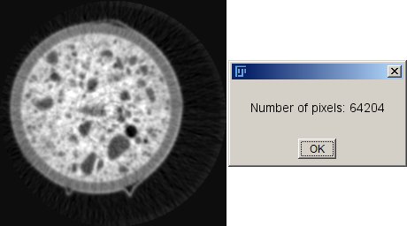
left: image i0, right: message box with number of pixel values >= 10
The code fragment
float value = 10f;
int[] mm = m0;
int anz = 0;
for (int ii = 0; ii < i0.length; ii++)
	if (i0[ii] >= value) anz++;
IJ.showMessage(" ", "Number of pixels: " + anz);
return new Object[] { mm, null };
left: image i3, center: image i5, right: image i5 embedded at the center area of image i3
Counts all pixels (or voxels) in the image (or volume) with a value larger or equal 10.
Or the code
int offx = (m3[0] - m5[0]) / 2;
int offy = (m3[1] - m5[1]) / 2;
float[] out = (float[])i3.clone();
for (int jj = 0; jj < m5[1]; jj++)
	for (int ii = 0; ii < m5[0]; ii++)
	out[ii + offx + (jj + offy) * m3[0]] =
		(i3[ii+offx + (jj+offy) * m3[0]] +
		 i5[ii + jj * m5[0]]) / 2f;
return new Object[] { m3, out };
takes the smaller image i5 and adds it to the center of the larger image i3.

left: image i0, center: image mask i1, right: message box with mean value of i0 within mask i1
The code fragment
double mean = 0;
int anz = 0;
for (int ii = 0; ii < m0[0] * m0[1]; ii++)
	if (i1[ii] > 127) {
		mean += i0[ii];
		anz++;
	}
mean /= anz;
IJ.showMessage("mean value: " + mean);
return null;
just calculates the overall mean value of image i0 within the ROI defined by i1 and displays it in a check box.

ramp image
Moreover, it is even possible to create your own images without any input image:
int mx = 256;
int my = 200;
float[] out = new float[mx * my];
for (int jj = 0; jj < my; jj++)
	for (int ii = 0; ii < mx; ii++) out[ii + jj * mx] = ii;
return new Object[] { new int[] { mx, my }, out };
creates an image containing a ramp (see image to the right),
circular mask
or,
int mx = 256;
int my = 200;
float[] out = new float[mx * my];
for (int jj = 0; jj < my; jj++)
	for (int ii = 0; ii < mx; ii++) {
		if (Math.sqrt(Math.pow(ii - mx / 2, 2) +
					  Math.pow(jj - my / 2, 2)) < 80)
			out[ii + jj * mx] = 255;
	}
return new Object[] { new int[] { mx, my }, out };
creates an image containing a circle mask in the center (see image to the right). For more information about the syntax, please consult the help function of the plugin itself.
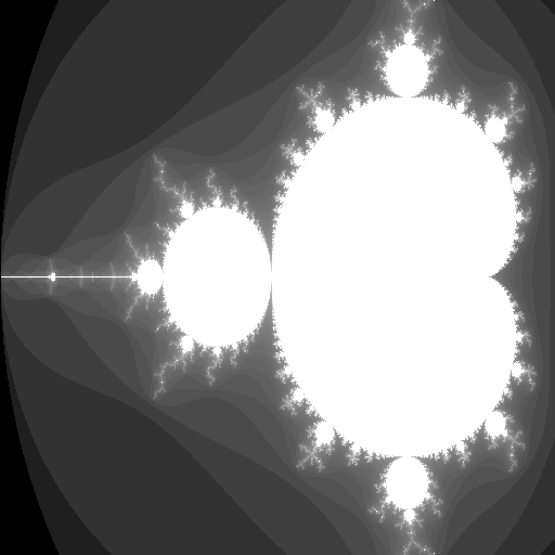
Mandelbrot fractal
As a final example, we show that it is also possible to create even more ‘cute’ images with that tool:
int max = 255;
int mx = 512;
int my = 512;
float[] out = new float[mx * my];
for (int jj = 0; jj < my; jj++)
	for (int ii = 0; ii < mx; ii++) {
		double px = -2. + (double)ii / 200.;
		double py = -1. + (double)jj / 255.;

		double zx = 0.0, zy = 0.0;
		double zx2 = 0.0, zy2 = 0.0;
		int value = 0;
		while (value < max && zx2 + zy2 < 4.0) {
			zy = 2.0 * zx * zy + py;
			zx = zx2 - zy2 + px;
			zx2 = zx * zx;
			zy2 = zy * zy;
			value++;
		}
		out[ii + jj * mx] = 50f * (float)Math.log(value);
	}
return new Object[] { new int[] { mx, my }, out };
This code fragment creates the image to the right showing a well-known Mandelbrot fractal!
Labeling 2D 3D
Particle analysis requires labeling of the previously determined particle mask which has been obtained by some type of image segmentation technique, e.g. by thresholding to mention the most simple one. The binary particle mask allows evaluation of the particles only globally. By labeling the particles, each particle is assigned a unique ID. Labeling is the prerequisite for evaluations considering local values such as particle size, diameter or other shape parameters on the single objects. This plugin implements the labeling of disconnected objects in both, 2D or 3D binary masks. The binarization from gray level images occurs via providing a lower and an upper threshold.
Particle image (left) and its labeling (right)
An example of labeling is given in the center and right images in the “Disconnect Particles” section, where the center image shows the particle mask before the disconnection procedure and before labeling. The disconnection procedure separates the single particles. After this step, the object mask is still binary and labeling is applied to colorize the particles in order to be able to distinguish them by their object values.
Median 2D 3D
This plugin supports conventional as well as geometric 2D and 3D median filtering for images and image volumes. The geometric median filtering is achieved according to the algorithm of E.V.Weiszfeld [Weiszfeld1937]. Unlike the conventional median filtering, geometric median filtering can be achieved for a multidimensional vector space rather than for a one-dimensional set of values only. That is, if multiple images exist at a single location, they can be filtered by using the common N-dimensional geometrical distance measure for finding the median.
Color image containing multiple phases (top left) and different types of median filtering: conventional band-wise (top right), multidimensional geometrical (bottom left), and multidimensional geometrical by choosing the closest available vectors.
The example color image (top right) shows multiple noisy phases. Conventional median filtering on each of the R,G,B bands separately yields the top right image. As can be perceived due to the RGB bands, new colors appear that are not present on the original image. Multidimensional geometrical filtering (in the RGB case, 3-dimensional) by using the Weiszfeld algorithm yields the bottom left image. When additionally confining to already existing color vectors only, the bottom right image results.
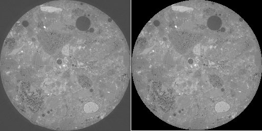
Remove Background
If an image is subject to consistent global shifts of the image values depending on the location, this might be due to inconsistencies in the data acquisition rather than to real changes in the material properties. In that case, background removal techniques might be appropriate. A typical example is image data from FIB-nanotomography (FIB-nt). Thereby, FIB-nt is applied onto cubes that are engraved into the flat sample surface prior to data acquisition. Due to shadowing effects, the subsequent 3D data acquisition lacks in loss of brightness and contrast towards the lower boundaries of the slices. This erroneously causes systematic inhomogeneities of the image values impeding reliable quantitative imaging. Correction of such deficits can be obtained by determining a global polynomial of low degree over the entire image and by subsequently subtracting the values of the polynomial function from the original image. The global polynomial function is determined by performing least squares optimization. Accordingly, systematic brightness variations can be globally corrected. The necessary assumption is that the overall image values remain more or less constant over the entire image, at least in an average sense.
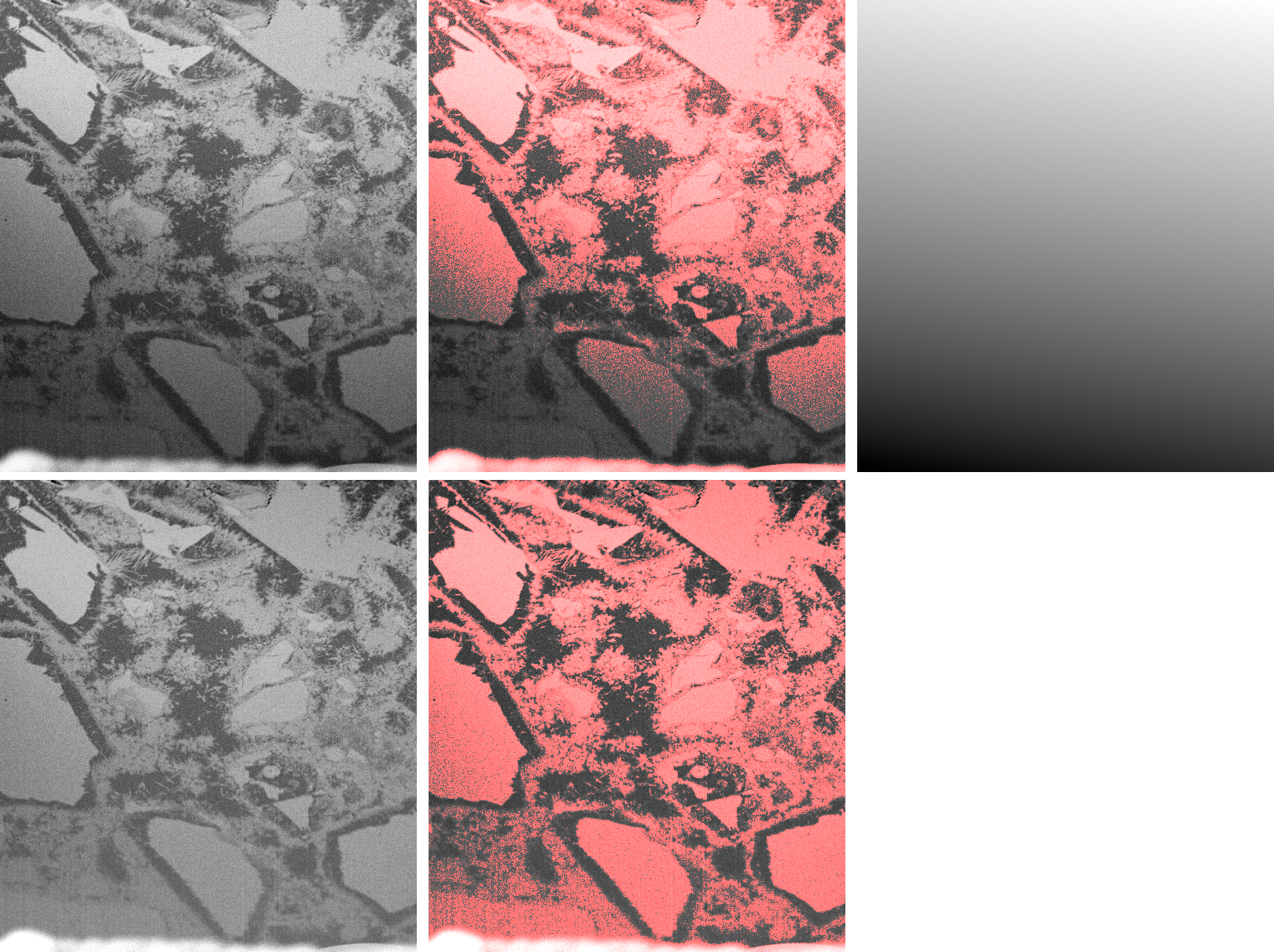
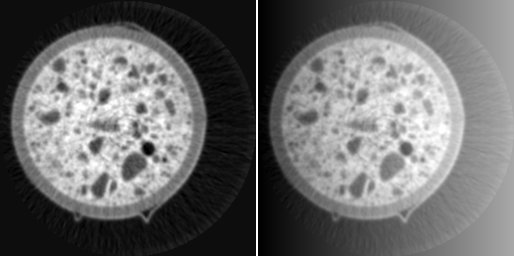
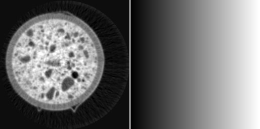
FIB-nt image with strong shadowing effects (top left), its thresholding (top centre), global polynomial of degree 1 (top right), its subtraction from the original image (bottom left), and its thresholding (bottom right).
An example from a FIB-nt image and its shadowing effects is given in the above figure (top left). After thresholding, the systematic brightness loss towards the lower boundary becomes obvious (top center). The determination of a global polynomial of degree 1 results in a background image (top right). After subtraction (bottom left), the brightness drop disappears, as subsequent thresholding (bottom right) approves.
In addition to the global homogeneization of the brightness values, the plugin also allows the correction of contrast values. However as an additional prerequisite, the image must be assumed to consist of a certain number of phases of more or less stable image values. In that case, a global polynomial can be calculated from the phase containing the lowermost image values, and a second polynomial from the phase containing the uppermost image values. The drifts are corrected by flattening both polynomial functions. The procedure hereby requires the number of phases as input parameter.
FIB-nt image of a fuel cell and its shadowing effects (left), and the image after correction (right) by assuming three existing phases.
The results of this kind of correction is displayed in the above figure. To the left, the original image is displayed. It consists of three different phases. Towards the lower border, a substantial drop of both, brightness and contrast occurs. Assuming a three phase image and after correction, the corrected image appears to be free from brightness and contrast drops (right).
Roundness 2D 3D
The roundness value of a connected object can be defined as the ratio of the actual size of the object and the size of the virtual sphere spanned by the largest diameter of that object.
2D: rnd = 4. * size / (diameter^2 * PI)
3D: rnd = 6. * size / (diameter^3 * PI)
Other well-known definitions (e.g. the definition of sphericity by Wadell [Wadell1935]) are based on the surface area of the sphere with the same volume as the object, relative to its actual surface area. The calculation of the surface area on pixelized objects is not straight forward, whereas the calculation of the volume size is just the number of object pixels or voxels. That’s the reason why we prefer the former roundness definition. Though, another useful option for pixelized objects could be the roundness definition of ISO which is based on the ratio between inscribed and circumscribed circles of an object, i.e. the minimum and maximum sizes for circles fitting inside and enclosing an object.
Roundness values are useful to provide a metric of how closely the shape of an object approaches a circle (2D) or a sphere (3D), thus for rating object shapes.
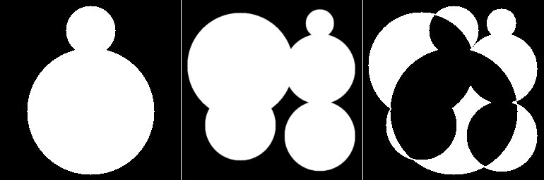
Skeletonization 2D 3D
In shape analysis, topological features can be captured from skeletons of the masks. Skeletons have several different mathematical definitions in the technical literature. Many different algorithms have been proposed. Many of them lack in retaining the original topology. A good conservation of the topology in 2D as well as in 3D was the main reason for the choice of the algorithm (Palagyi, [Palagyi1998]). This feature is displayed in the figure below, where a set of geometrical 3D objects is provided (left). After skeletonization (center), the topology is mainly being preserved. If the diameter of the skeletoized pipes is inflated up to the values from the distance transform of original volume (right), the thus restored objects obtain high similarity to the original ones.
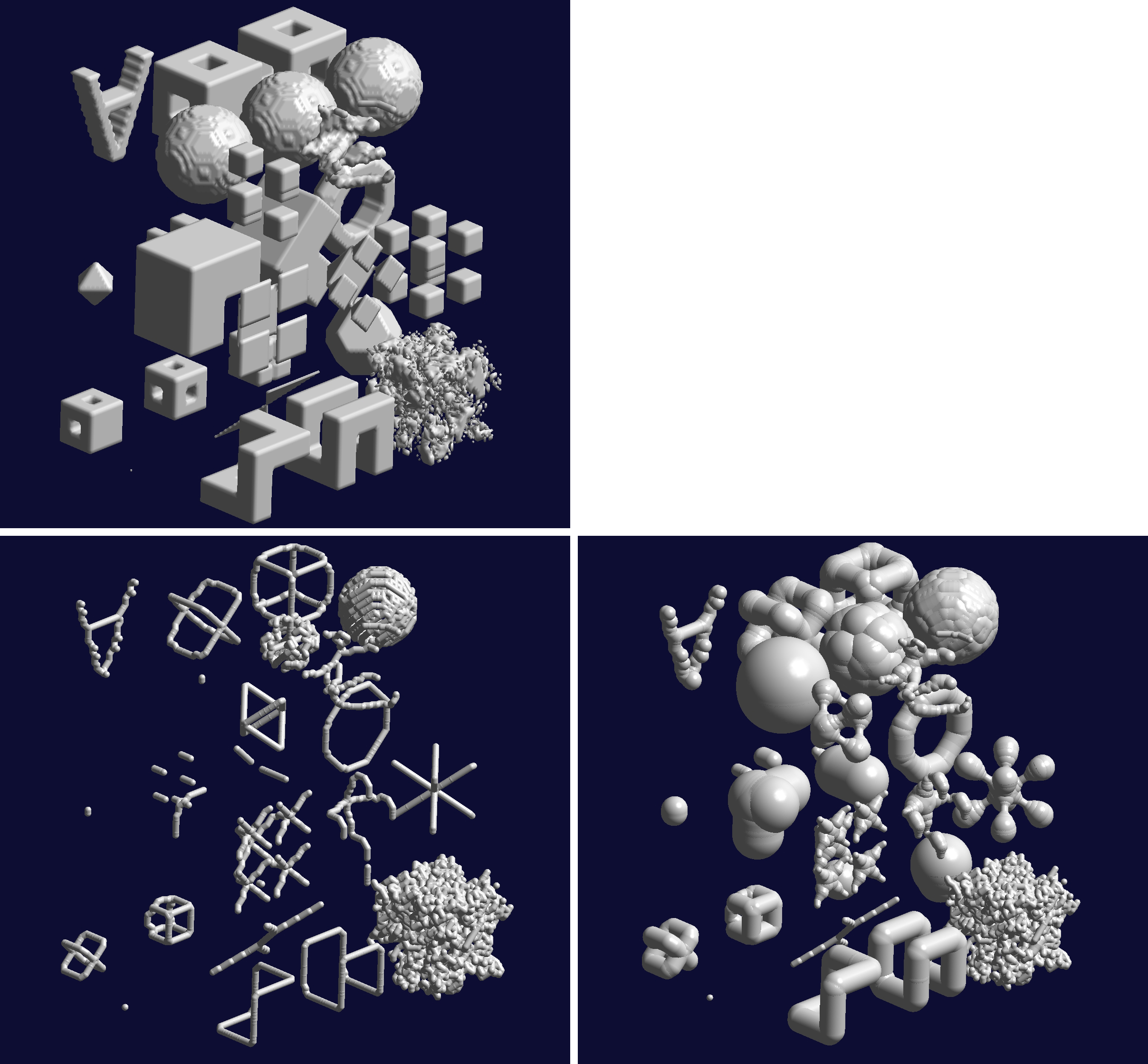
Some 3D objects (top), their skeletonization (bottom left) and their restoration by inflating the pipes up to the distance transform values of the original objects (bottom right).
Stripe Filter
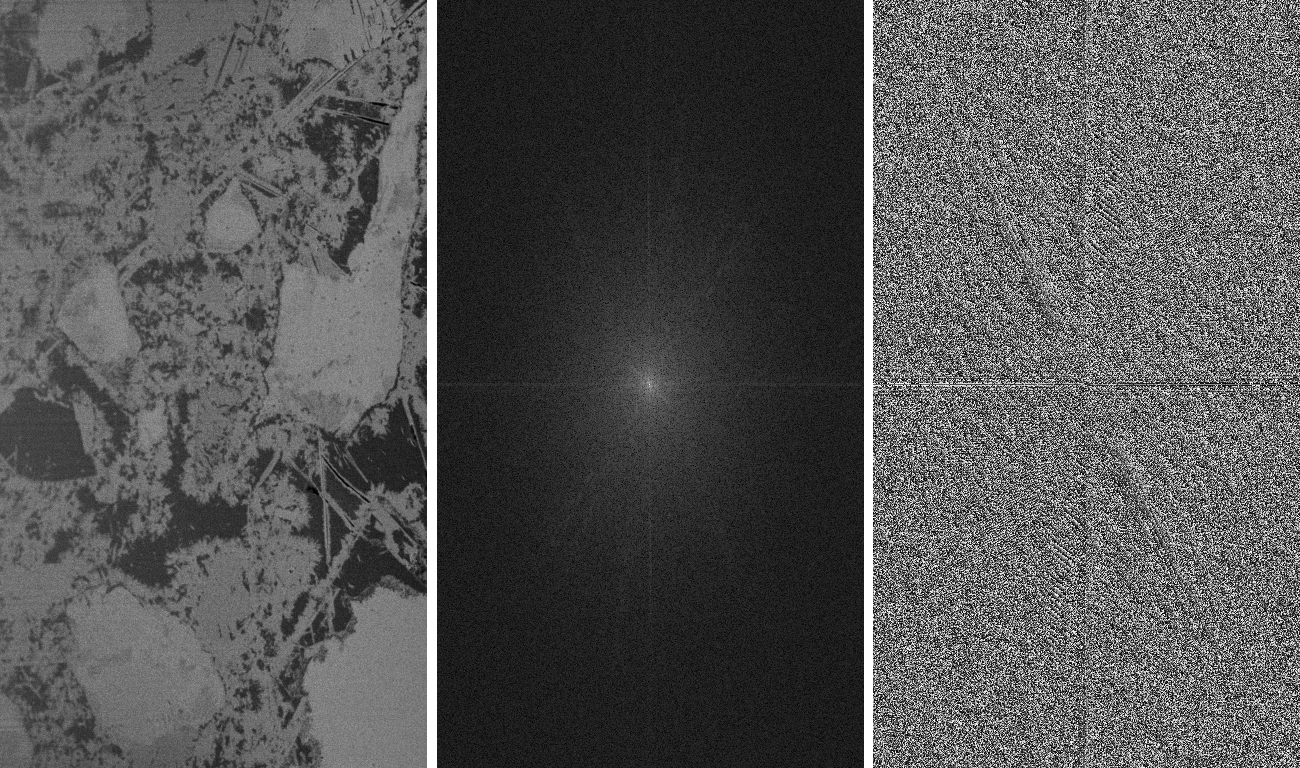
Striping artifacts may occur due to undesired effects during data acquisition. Defect detector pixels might be the reason of stripes in the projections of computed tomography measurements resulting in ring artifacts after reconstruction. Waterfall artifacts might be the reason for stripes when accessing 3D data using FIB-nanotomography. Both types of artifacts can be erased by a technique for stripe filtering based on the combination of wavelet and Fourier transform [Münch2009]. The potential of the stripe filtering plugin is shown in the figure below by applying it to a gray level image (top) and to a RGB image (bottom).
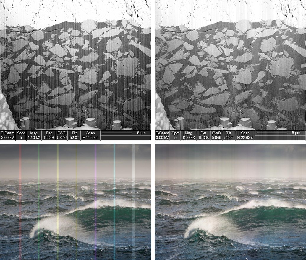
Gray level (top) and RGB (bottom) image containing horizontal stripes (left) and the results of the stripe filtering plugin (right).
In the next figure, the stripes in CT projections (top) and the resulting ring artifacts in the reconstructed images (bottom) is presented, the original situation to the left and the results after stripe filtering to the right.
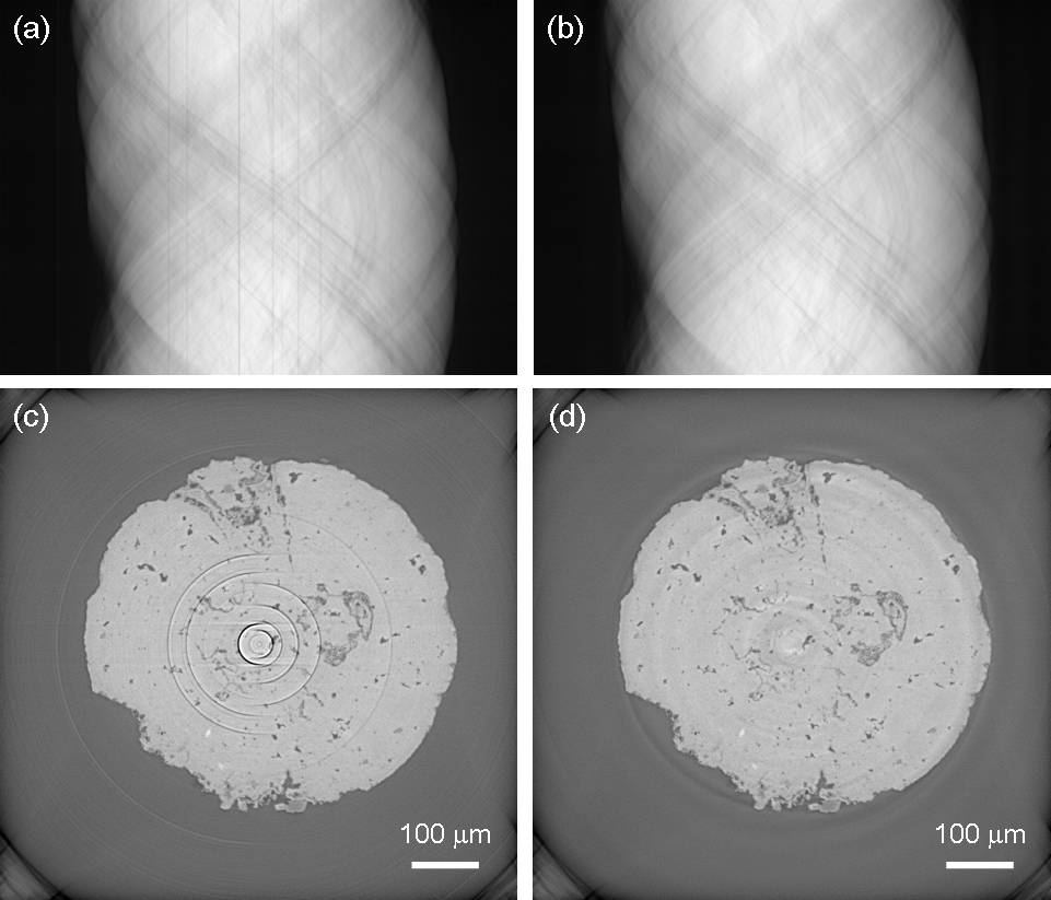
Projection image in a CT slice (top) before (left) and after (right) stripe filtering. The stripes in the projections yield ring artifacts in the reconstructed image (bottom). An original (left) and its filtered version (right) is displayed.
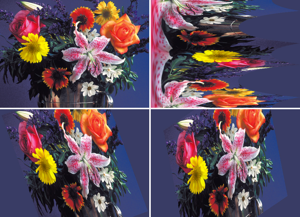
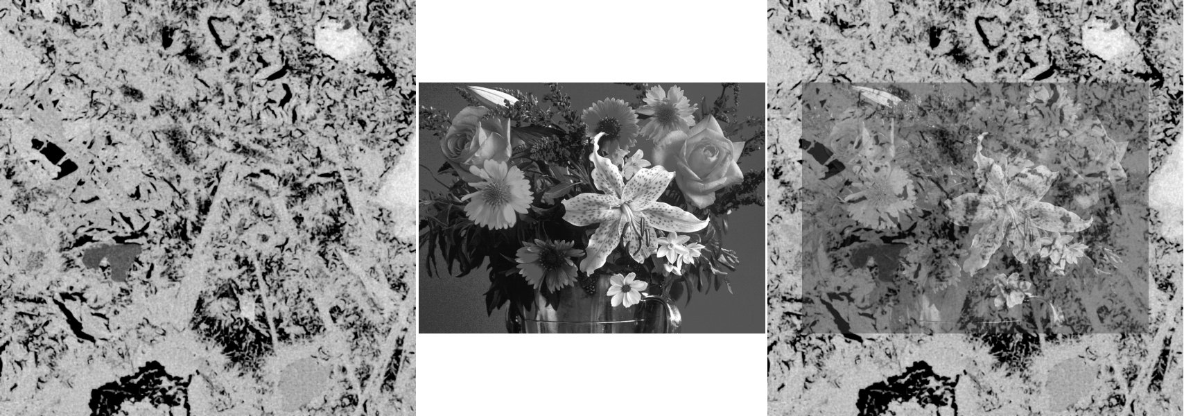
Flowers image (top left), its transform into polar coordinates (top right), its scaling followed by a rotation (bottom left), its rotation followed by a scaling (bottom right).
Transform 2D 3D
This plugin provides image transforms for 2D images and for 3D image volumes by using polynomial fits of arbitrary degree. Various transforms can be chosen, including translation, rotation, scaling in arbitrary order and by choosing variable centrum coordinates.
This can be performed by using an operations strings syntax containing translation (‘t’), rotation (‘r’) and / or scaling (‘s’) operation(s). Each operation is followed by its comma separated translation, rotation or scaling values. For instance, an operation
t10,-20r30
defines a translation by (10, -20) followed by a rotation by 30 in degrees in 2D around the original center point. Likewise,
s0.5,0.8,1.5p0,0,0r-10,20,30t11,-22,33
defines a scaling by (0.5, 0.8, 1.5) followed by a rotation by (-10, 20, 30) in degrees around (0, 0, 0), followd by a translation by (11, -22, 33) in 3D.
The corresponding homogeneous 4x4 (for 3D, or 3x3 for 2D) matrix operation is always indicated on the fly. Of course, the specification of the 4x4 (or 3x3) homogeneous matrix itself is possible as well. Moreover, the transformation of cartesian to cylindrical or spherical coordinates or vice versa is supported. Also, resampling into another pixel size is feasible.
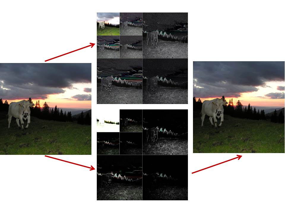
Cow at Swiss alps (left), its wavelet decomposition at decomposition level 2 by using the Haar wavelet when providing a nice view (top center) and a reconstructible format (bottom center), and finally, its reconstruction (right).
Wavelets 2D
This program provides wavelets decomposition and reconstruction of 2D images. The decomposed set of wavelets can be chosen to be either reconstructible or non-reconstructible, i.e. just for visual presentation. If it is selected to be reconstructible, the image quality might be not really perceptionally ideal for presentation purpose. Hence for creating more attractive wavelet images, the choice of non-reconstructible wavelets might be preferred. The term “non-reconstructible” means that the sets of wavelets are normalized and cropped at the boundaries and therefore miss information for proper reconstruction. In the case of color images due to the restricted color resolution (8 bits per channel only), reconstruction might be feasible, however, the results usually are far beyond acceptable quality. Therefore for color images if reconstructability is required, we recommend splitting into R,G,B channels and processsing of each channel separately in order to achieve floating point rather than 8 bit resolution.
After a wavelet decomposition, the wavelet specifications (e.g. “db2” for the Daubechies 2 wavelets) together with the normalization parameters (boundary handling, output normalization) are stored to the image as additional info. Thereby if a wavelet decomposition is saved to TIFF image file format, this additional image information is being stored to the image file header. Consequently, the respective wavelet settings will be automatically recovered when the wavelet plugin is launched to such image.
The example to the right shows a Haar wavelet decomposition of an image. A graphically nice (top center) as well as a reconstructible version (bottom center) is presented. Reconstruction (right) is possible only from the reconstructible version. Since colour images are usually resolved with 8 bits per R,G,B-channel only, the reconstruction is not perfect but still acceptable for this example. In contrast, gray level images result in wavelet decompositions in floating point format and therefore allow perfect reconstructions.
Reconstruction
Plugins of this section support preprocessing and reconstruction of images from projection data for CT imaging.
Another category of methods in this section is the estimation of 3D data from 2D images with the idea of estimating parameters requesting 3D connectivity from 2D slices only.
Filtered Backprojection
This plugin provides convolution / backprojection of a set of projections to an image. It supports different reconstruction filters (Shepp & Logan, Parzen, Hamming, Hann, Rectangular). The sequence of angles as well as the sequence of the projections can be altered.
Projections Sinograms
This plugin converts sets of projections into stacks of sinograms and vice versa. It also supports flat and dark field correction, speckle filtering, Lambert inversion, adjustment of the rotation center, re-ordering of the projections, adjustment of the value range, etc.
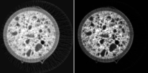
Reconstruct 3D from 2D
This plugin provides the reconstruction of virtual 3D phase volumes from 2D phase images. The goal is to preserve the structural characteristics given in the 2D image and to extrapolate it to 3D.
The algorithm assumes that the 2-point autocorrelation function of similar structures is being preserved. The essential idea is to solve the 3D-reconstruction problem time efficiently in the Fourier space by applying the Wiener-Khinchin theorem. Basically, the autocorrelation function of the 2D image is extended to 3D and Fourier transformed. In the Fourier space, the arguments of the complex values are randomly chosen while keeping the magnitudes. Inverse Fourier transform then yields the newly estimated 3D volumes.
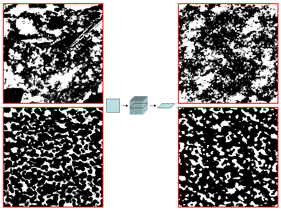
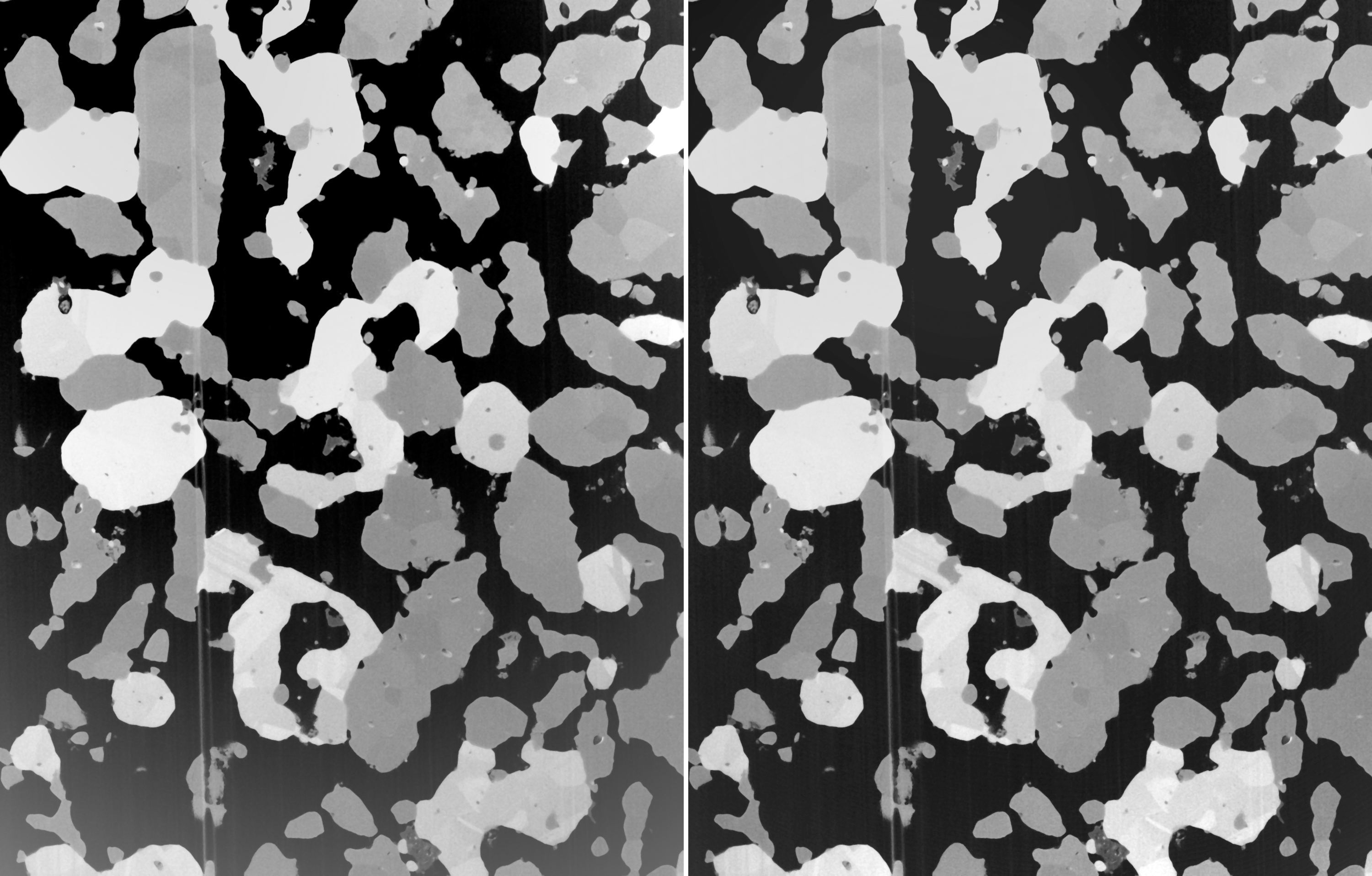
Segmented masks from cement paste (top left, OPC CEM 1, 42.5, w/c 0.35, 28 days hydration) and from the contact zone of the anode membrane of a solid oxide fuel cell (bottom left). A virtual 3D reconstrucion was applied to the original structures (center). A single slice from the 3D image stack is displayed for both cases (right), showing different structures than the original ones, with however closely resembling characteristics.
Examples of the 2D-to-3D reconstruction are given in the figure above for a structure from cement paste (top left) and for a structure from a solid oxide fuel cell (bottom left). The original gray level images have been acquired by SEM (scanning electron microscopy) at a pixel resolution of 20nm. Segmentation has been achieved by thresholding. After reconstruction of the 3D stack, a single slice of the reconstructed volume is displayed (right), revealing a “similar” structural appearance as the original one. The shaded surface of the reconstructed 3D mask is presented in the figure below for the cement (left) and the fuel cell (right).
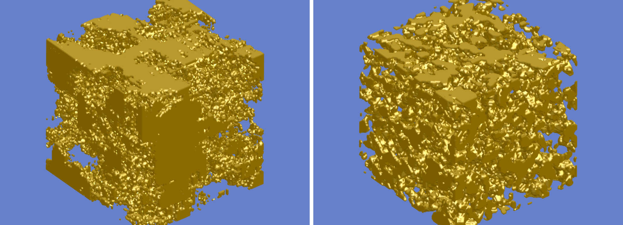
Shaded 3D representation of the reconstructed 3D stacks from the reconstructed volume of the cement paste (left) and the anode membrane (right).
Evaluation
The plugins of this section achieve quantitative evaluation on image values and structures. This is an important topic in image processing in different scientific fields. A result from quantitative evaluation is not an image as it is from filtering, but rather a number representing some structural characteristics.
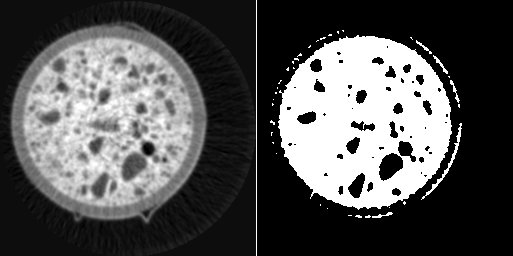
Particle Size Distribution
This plugins calculates the particle size distribution (PSD) from a stack of images containing already segmented and labeled particles [Münch2006]. Either single images containing 2D particles, or stacks of images representing 3D volumes can be processed.
The following features can be calculated:
- particle ID
- particle volume
- cumulative particle volume
- particle surface area
- cumulative particle surface area
- mean particle radius
- number of particle borders
- particle count
- cumulative particle count
- particle count weighted according to the number of boundaries
- cumulative particle count weighted according to the number of boundaries
- boundary value in case of clustering
- cluster mean value in case of clustering
Correction of particles that are clipped at the borders is also possible. The correction is applied to the resulting pore radii only (i.e. not for the pore volume). The plugin allows cumulative integration of the particle volumes and surfaces starting from either small or large particles. The program plots out the resulting parameter fields.
Per default, the function plots a parameter set for each particle separately. Additionally, the program allows different types of clustering of the parameter sets. Clustering means summing up or averaging the parameters within intervals yielding a histogram.
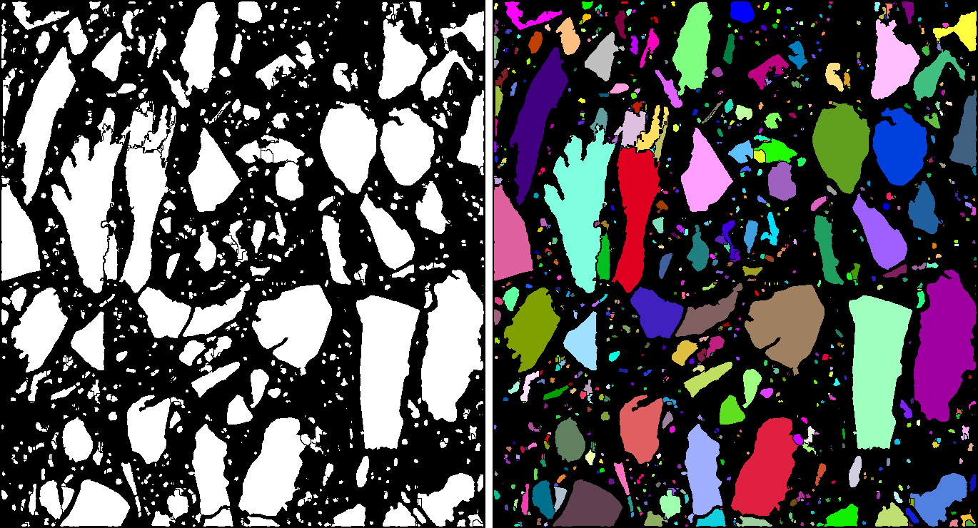
An example of a 2D particle image, of its mask and some particle evaluations is given in the figure below.
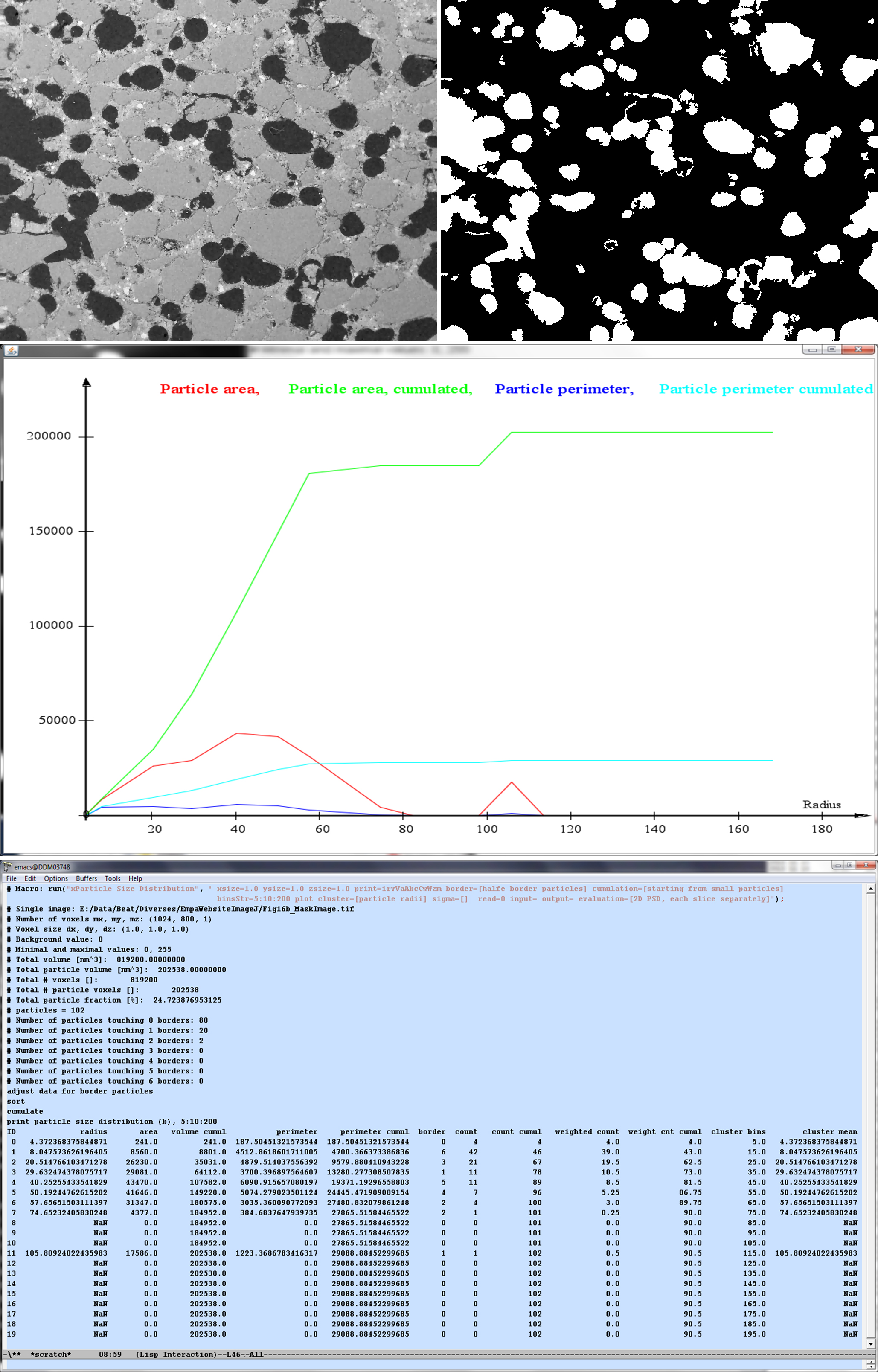
Grainy structure (top left), segmented mask of the grains (top right), and the evaluation of its particle size distribution (center and bottom).
Phase Image Evaluation
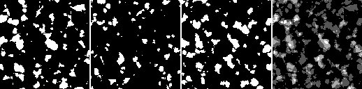
This plugins provides an evaluation of phase images [Leemann2006, Leemann2010] containing labeled phases. For instance, labeled images might be created interactively with the help of the plugin “Segment Phases 3D”, or even automatically with the plugin “Cluster Image”.
The phase image evaluation calculates some parameters of all phases, including the percental phase contents and the phase areas. Additionally, mean image values for each phase can be provided, if one or more gray value images associated to the current phase image are provided.
Furthermore, the plugin supports a peeling evaluation. Peeling starts from a specifically defined phase to its surroundings and requires a set of peeling radii defining toroidal regions around the starting phase. The peeling evaluation yields a data line at each peeling radius, including the peeling distance, number of pixels, mean value, and the percental phase contents for each phase. For image stacks, true 3D evaluations can be performed.
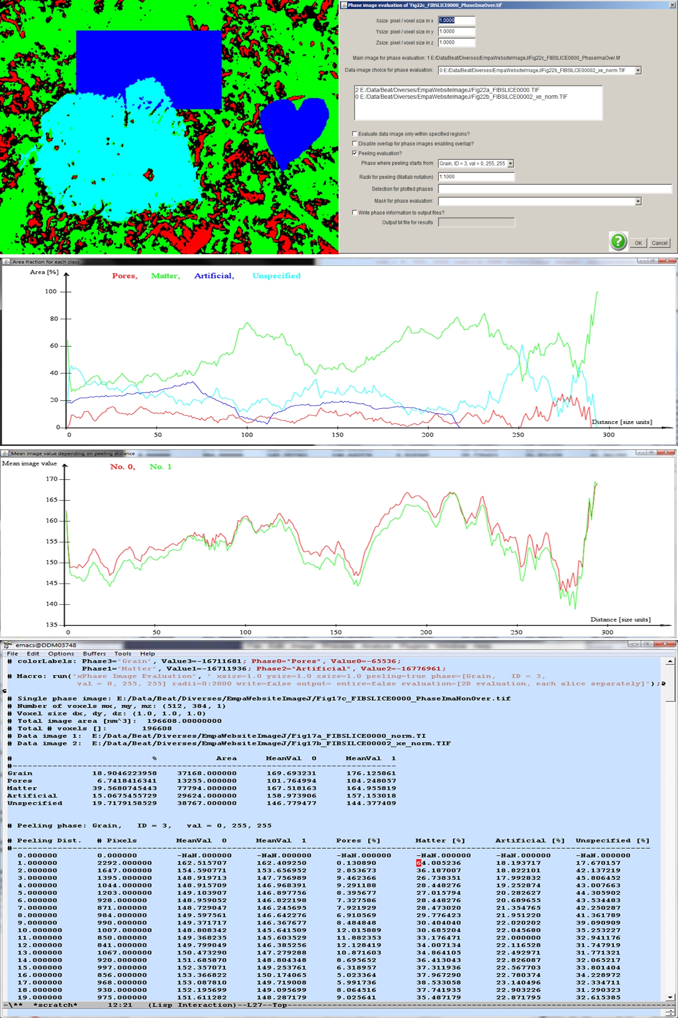
Phase image (top, left) and the parameters provided for the phase image evaluation (top, right). The resulting plots and the list of parameters are displayed below.
An image defining some phases is given in the above figure (top, left). The cyan colored center particle is supposed to act as the location from where peeling is initiated. The percental areas of the phases “Pores”, “Matter”, “Artificial” and “Unspecified” are plotted below. As it is evident from the calling parameters (see above figure, top, right) two gray level data images associated to the pore mask are provided (center field). Their mean values depending on the peeling radius are displayed in the graph at the bottom. The parameters are provided in a text file as well (bottom).
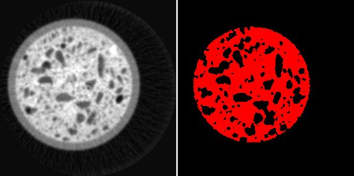
Pore Size Distribution
This plugins calculates the pore size distribution (PSD) for a pore structure [Münch2008], i.e. the distribution of the pore radii. The PSD can be calculated either in 2D or in 3D if the program is running on a stack of images. The pore masks must be prepared beforehand such that a simple thresholding procedure is capable to separate the locations of the pore from the material. The PSD calculation will be running on the pore phase.
PDS’s can be defined in different ways and must be chosen according to the specific requests [Münch2008]. The following PSD types can be calculated:
- Discrete PSD: the generally used definition of a PSD from image data. The pores are regarded as discrete object. At each single pore, its pore area or pore volume is calculated and the radius of its circle- or sphere-equivalent object given.
- Continuous PSD: the pore space is categorized into regions of different radii in the sense that the regions can be filled with balls of different radii. The sizes of those radii are then attached to the respective locations. The histogram of radii then acts as continuous PSD.
- Continuous PSD with MIP simulation: same PSD definition as for the continuous PSD. However, the balls of different radii are intruded into the pore volume from one of the faces of the image cube (3D), or from one of the edges of the image (2D), respectively. This definition of the PSD corresponds to the pore size data that is retrieved by mercury intrusion porosimetry (MIP).
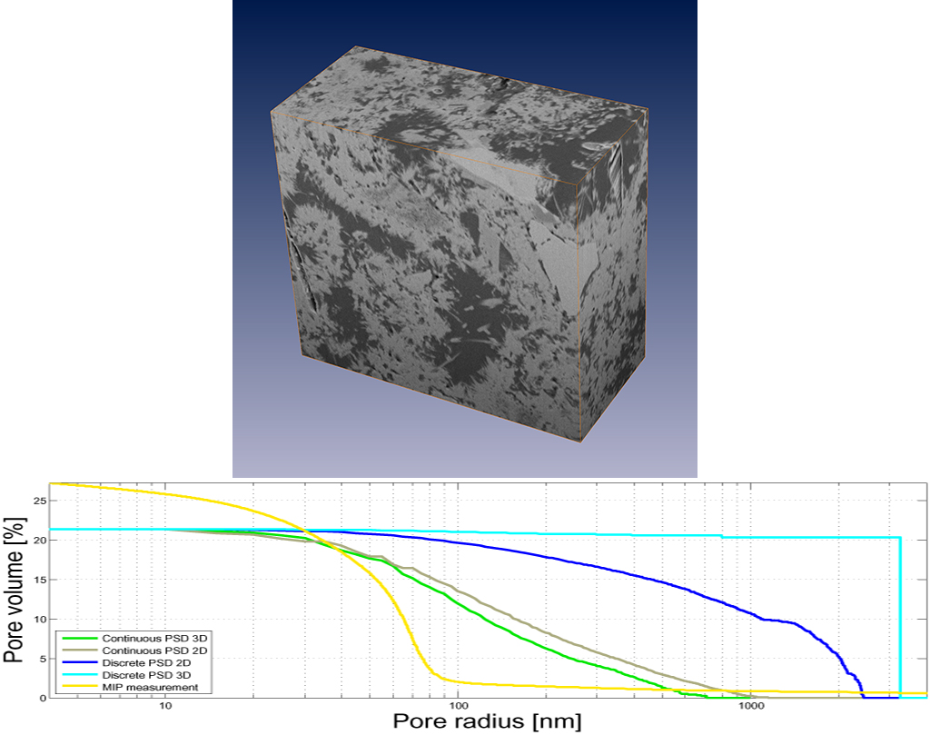
3D volume of cement paste (OPC CEM 1, 42.5, w/c 0.35, 28 days hydration) acquired by FIB-nanotomography (top) and its pore size distributions of varying definition (bottom, see referenced paper).
The above figure (top) shows a picture of a 3D volume of cement paste measured by FIB-nanotomography at a pixel size of 14.84 x 18.84 x 30.0 nm^3. The pores have been segmented by thresholding and different definitions of PSD’s have been calculated in slice-wise 2D as well as in real 3D (bottom graph, containing the results of the PSD calculations visualized by MATLAB).
Editors and Viewers
This section contains plugins that are designed for user-interactive visualization and data processing on 2D slices and 3D volumes. They therefore don’t just support a unique interaction on some image data, but they provide engines supporting an interactive dialog between the computer and the user.
Display Volume
This plugin provides an orthogonal slicer for image volumes. The top view (xy), front view (xz) and side view (yz) of the volume are displayed at a specific point, the center point at startup. The point then can be moved by mouse interaction in one of the views while the remaining views keep track of the changes. Thereby, any x,y,z-location in the 3D volume can easily be focused and displayed. The image value at the current position is always plotted to the ImageJ window.
As soon as the plugin is activated, the respective image stack disappears. Likely, as the orthogonal slicer window is closed, the respective image stack reappears again and the current slice position is selected.
As the plugin is activated, the orthogonal slicer acts like a common image stack, that is, any filter operations or plugins can be applied to either a single slice or to the entire volume. One of the restrictions is that overlays cannot be handled with this plugin and like this, selection of ROIs (i.e. with the selection tools) are not supported.
Tip: if you add a shortcut for the “Display Volume” plugin, it is easily possible to switch back and forth from a conventional image stack to an orthogonal slicer and vice verca.
|
Orthogonal slicer view of the nanotomographic 3D volume from cement paste as displayed in the section for the “Pore Size Distribution” plugin (top). |
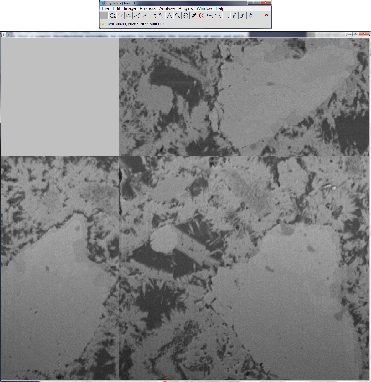
As an example, the above figure displays the view of the orthogonal slicer applied to the 3D volume displayed in the “Pore Size Distribution” section (top). The red cross-lines of the slicer show the current 3D cursor position which allows interactively focusing any point in the 3D space. The position vector and the associated image value are plotted to the ImageJ window (top).
Edit Label Region
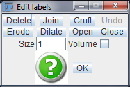
This plugin provides an engine for interactive editing of label images or label volumes (i.e. stacks of images). Label images are images holding a set of regions at one specific gray level or color per region (example see figure in “Disconnect Particles”, right). Operations such as deleting, joining, eroding, dilating, opening, or closing of manually selected 3D objects are supported. There is also an operation for deleting objects smaller than a certain size. For stacks of images, all operations can be performed either in slice-wise 2D, or truly volumetrically in 3D. The interface of the engine is visualized in the figure to the right.
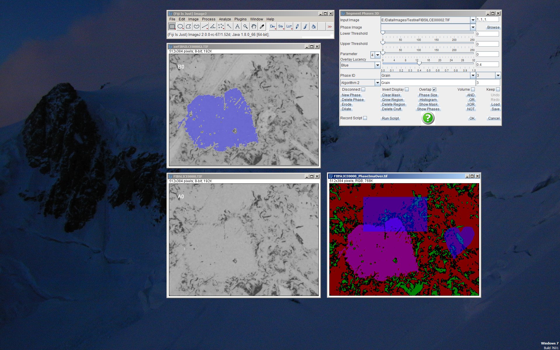
Engine for 3D segmentation (top right) which is currently operating on two gray level images (left). The image at the bottom right is the interactively segmented phase image which is currently containing four different phases (see top left figure for the plugin “Phase Image Evaluation”).
Segment Phases 3D
This plugin provides an engine for interactive segmentation of multiple phases. The program works on both, single images as well as image stacks. For image stacks, the operations can be performed in either slice-wise 2D or in 3D. All images or image stacks currently opened in an ImageJ session may serve as input images or image volumes. This benefit of being able to use multiple input images enables creating phase masks from multiple coincident or from multiple filtered versions of the same 2D or 3D scene. The plugin is designed for interactive use, however it provides a scripting language enabling to run scripts in non-interactive mode. Thus, automated segmentation processes can even be launched from command line.
The output of this program is a 2D phase image or a 3D phase stack of images which may contain up to 24 different phases. A phase is created by defining a bit mask by using different types of operations on any of the input images. Possible operations for building a phase include manual drawing (by using the selection buttons on the ImageJ main toolbar), thresholding, regular or constrained region growing, erosion, dilation, and removal of small regions.
An intelligent workflow allows progressive refinement of each single phase represented by its bit mask. The bit masks are being interactively modified by using logical arithmetic (i.e. Boolean AND, OR, XOR, NOT) on a) the already present bit mask and b) the temporary mask created by one or more of the operations listed above. If, for instance, a thresholding operation was selected, its temporary mask can be added to the currently selected phase by running an “OR” operation. A temporary mask during an operation is always distinguished by its red color, while the currently valid mask after completion of the operation is denoted by its blue color.
A phase name and an ID are assessed to each phase for later processing. The ID is important in the case some phases may overlap each other, in order to define the priorities.
The resulting image may be either a simple binary 2D or 3D mask of the currently selected phase (button “Show Mask”), or it may be a phase image or image stack consisting of a 32-bit color TIFF image holding multiple phases (button “Show Phases”). In the case of a phase image containing multiple phases, each phase is denoted by a single bit from the 32-bit integer number. Thereby, all phase names and ID’s are additionally being stored to the TIFF file header. Hence, a thereby created TIFF phase image can be later re-loaded for further processing together with all their intrinsic phase names.
For understanding the basic principle of working, consider the following example steps:
- Select the requested image by clicking with the mouse on it, then go back to the “Segment Phases 3D” tool and click on the GUI. Like this, the requested image is being activated. Alternatively, the currently active image can be selected with the combo box “Input Image”
- For thresholding an image and thus by defining a binary mask, select a value range by adjusting the lower and upper thresholds. This can be achieved by either moving the sliders or by typing the values to the text boxes to the right (and confirming with
). A red temporary mask appears as an overlay. - Likewise, temporary masks can also be created by using the ImageJ tools “rectangle”, “oval”, “polygon” or “freehand” selections (in 3D mode, applies to slices only).
- Press the button with the requested bit operation for applying the temporary mask to the currently valid mask. For instance, if the currently valid mask is empty as always when starting a new session or when defining a new phase, an “OR” operation adds the temporary mask to the current void mask. A blue resulting mask appears.
- As soon as the current mask (blue) is not void, bit operations “AND”, “XOR” or “NOT” can be likewise applied by combining the current blue mask with a newly generated red temporary mask.
- For image stacks, this (or any other) operation is either performed in 2D or in 3D depending on whether the “Volume” checkbox is checked.
- Both, current as well as temporary mask can be further refined by applying region growing, erosion, dilation, or small particle removal operations (button “Delete Cruft”). Thus, any of those operations can be applied either to the red mask prior to applying a bit operation, or to the currently valid blue mask.
- The “Grow Region” and “Delete Region” operations require one or more initial points that can be defined using the “point” or “multiple-point” tool of ImageJ. In Addition, the “Grow Region” process can be constrained by the minimal size of the pixel neighbourhood which is defined by the slider and the text field “Constraint”.
- Both, the “Erosion” and Dilation” operation tools require the erosion or dilation size to be defined by the “Size” text box.
- The “Delete Cruft” tool for removing small particles requires the maximal size of the particles that should be deleted. This is achieved by defining the numbers with the “Size” text box.
- A simple binary mask of the currently selected phase can be retrieved by pressing the “Show Mask” button.
- Most of the editing steps can easily be annulled by using the “Undo” button. Recovering an annulled editing step is also possible by using the “Redo” button. Like this, up to 32 editing steps can be restored.
- If more than one phases should be defined, each phase can be individually created by pressing the button “New Class”. A new class obtains an initial name that can be manually overwritten (press
key after editing). Each class layer can now be separately edited after it was selected by the "Class ID" combo box. Removing of the current class is achieved by pressing "Delete Class". - By default, phase classes are overlapping each other by following the hierarchical descending order inherent to the “Class ID” combo box to the right. This hierarchical order can be altered by changing the numbers in the combo box to the left (by writing the new numbers to the text field followed by pressing
). Alternatively by checking the check box "Overlap", the phase classes can be specified to independently overlap each other. If overlap mode is specified, the phase hierarchical order is irrelevant. - Phase images are coded as RGB color images. Already existing phase images can be loaded by opening them with ImageJ and then by defining them by the respective entry in the combo box “Phase Image” followed by pressing the “Load” button. Alternatively, they can be opened and loaded by choosing the file path by using the button “Phase Path”. If not yet existing and by pressing “Show Phases”, phase images are being created. If open and displayed, they are updated after each modification of any of the classes they include. By pressing the button “Save”, the current version of the phase image is being saved, by default to the path selected in “Phase image”.
- Due to additional event listeners, an open “Segment Phases 3D” instance raises the time that is needed when browsing through the slices of an image stack. This blocking effect might be annoying. In order to bypass the listeners and thus to enhance the speed, the check box “Disconnect” might be temporarily checked (and unchecked, if “Segment Phases 3D” is being used again).
- By checking the check box “Record Script”, a text editor is opened and each performed action recorded. The created text file can later be adjusted, stored to file, reloaded and be run by pressing the button “Run Script”.
The segmentation engine is visualized in the figure to the right while operating on two SEM images of cement paste (OPC CEM 1) acquired at the same location but at different microscope settings. The color image to the bottom right shows the currently constructed phase image consisting of 4 different overlapping phases. The same image in non-overlapping mode is displayed in the section for the “Phase Image Evaluation” plugin, top left. Currently, the phase named “Grain” is active and overlayed to the top left gray level image in transparent blue. Like this, any current operation would now be achieved to the “Grain” phase. The rectangle and heart shapes were drawn manually with the selection tools.
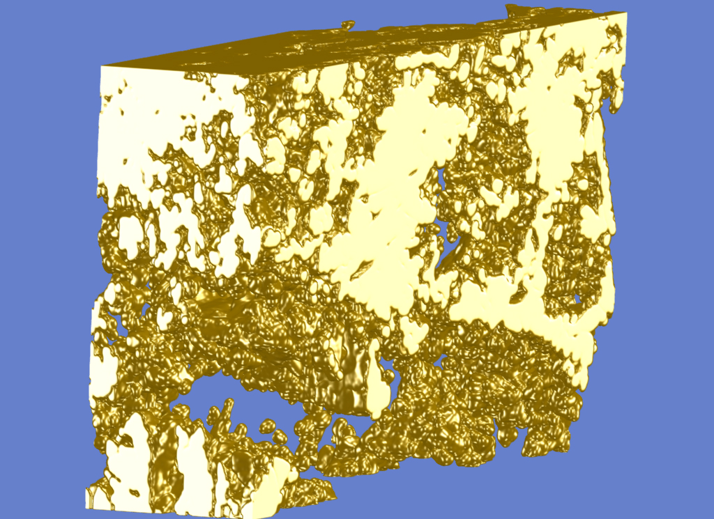
Triangulated and shaded visualization of the 3D volume in the plugin for “Pore Size Distribution” and “Display Volume”.
View 3D Mask
This plugin provides a 3D viewer of image and skeleton masks. The original data base should be a stack of images. An image mask may contain the mask of arbitrary objects, while skeleton masks should contain objects which are previously skeletonized in 3D. 3D skeletonization can be performed by previously calling the “Skeletonization 2D 3D” plugin.
For 3D shading, the image masks can be either triangulated or voxelized. The triangulation is performed by using the well-known marching cubes algorithm [Lorensen1987], while voxelization is performed by a technique of Artzy et al (see reference below).
The viewer is resizable. The 3D scene can be rotated, translated, or scaled. Rotation can be achieved with the left mouse button. Translation in x, y can be achieved by the right mouse button. Translation in z is sometimes useful if the viewer is too close to the scene. It can be achieved by the middle mouse button. Scaling is achieved by simultaneously pressing down the
The current transform matrix is always stored to a text file located in the folder from where ImageJ was started. It is updated after each change of the rotation, translation or scaling. Like this, the current settings of the scene that seem to be useful for further visualizations can be stored to file.
The 3D viewer also contains a button to the bottom called “save canvas as JPEG”. By pressing it, the current view can be stored to JPG image. The resolution of this image corresponds to the current resolution of the 3D window, i.e. to its window size.
As an example, a triangulated view of the segmented 3D volume is presented in the image to the right (see nanotomographic 3D sample from cement paste, image of plugins “Pore Size Distribution” (top image) and of “Display Volume”). Other examples were given in the plugin description for “Reconstruct 3D from 2D” and for “Skeletonization 2D 3D” showing the original 3D scene, its skeleton and its skeleton after resizing its elements to their size determined by the distance transform values (see “Distance Transform” plugin).