TrackMate Performance

This is a very incomplete DRAFT

The test machine

The computer used for these tests is the following:

• Mac Pro
• mi-2010
• Processor 2 x 2.66 GHz 6-Core Intel Xeon
• Memory 24 GB 1333 MHz DDR3 ECC
• Software Mac OS X Lion 10.7.5 (11G63)

Time of execution

The tests reported here were run on an Apple Mac Pro, 2 x 2.66 GHz 6-Core Intel Xeon, 24 Go 1333 MHz DDR3, running Mac OS X v10.7.5, with Java 1.6. The detectors instantiated were tamed to use only 1 thread. Unless indicated, the median filter and the sub-pixel localization were not done.

The DoG & LoG detectors

Processing time for a 2D image as a function of its size

For a uint16 image, varying its size, containing 200 gaussian spots of radius 3 (everything is in pixel units).

N (pixels)	Image size	DoG detector time (ms)	LoG detector time (ms)
256	16x16	3.0	4.8
1024	32x32	2.95	4.3
4096	64x64	3.95	4.35
16384	128x128	7.9	5.85
65536	256x256	23.35	17.7
262144	512x512	88.2	61.15
1048576	1024x1024	357.3	251.65
2359296	1536x1536	789.85	605.4
4194304	2048x2048	1463.4	1201.1

For the DoG detector, unsurprisingly, we find that the execution time is proportional to the number of pixels, following approximately t (ms) = 3.4e-4 x Npixels. This is expected as all calculations are done in direct space.

The LoG detector operates in Fourier space, and because of the Fourier transform implementation we use, the images are padded with 0s to reach a size equal to a power of 2. This does not show here as all but one tests are made with such a size. Still, the execution time slightly deviates from the linear case, and shows a slight quadratic shape. The best linear fit yields a low in t (ms) = 2.8e-4 x Npixels, showing that the LoG detector is slightly quicker than the DoG detector.

Processing time for a 3D image as a function of its size

N (pixels)	Image size	DoG detector time (ms)	LoG detector time (ms)
4096	16x16x16	8.7	24.7
32768	32x32x32	23.5	38.5
262144	64x64x64	129.3	159.2
2097152	128x128x128	875.1	936.3
16777216	256x256x256	7054.0	7462.4
134217728	512x512x512	61477.2	58860.6

And again, the processing time is found to be linear with the number of pixels. The linear fit is slightly steeper, however: t (ms) = 4.6e-4 x Npixels, which we attribute to the 3D kernel overhead.

Interestingly, the LoG detector seems to become the slowest at intermediate size, which I cannot interpret well.

Processing time for a 2D image as a function of the spot radius

We used a 1024x1024 uint16 image, with 200 gaussian spots, the size of which we varied. The detector was tuned to this radius.

We find that for the DoG detector, the processing time to increase linearly with the specified radius, following approximately t (ms) = 20.5 x radius + 260. As the difference-of-gaussians is calculated in the direct space, a marked increase is expected as there is more pixels to iterate over. Without optimization, we should however have found the time to be increasing with the square of the radius, and find the same dependence that for the image size. Thanks to the clever implementation of gaussian filtering¹, this is avoided.

The LoG detector shows a near-constant processing time, which makes it desirable for spots larger than 2 pixels in radius. This is due to the way we compute the convolution which is explained below.

Processing time for a 3D image as a function of the spot radius

This time we used a 256x256x256 3D image, but with otherwise the same parameters.

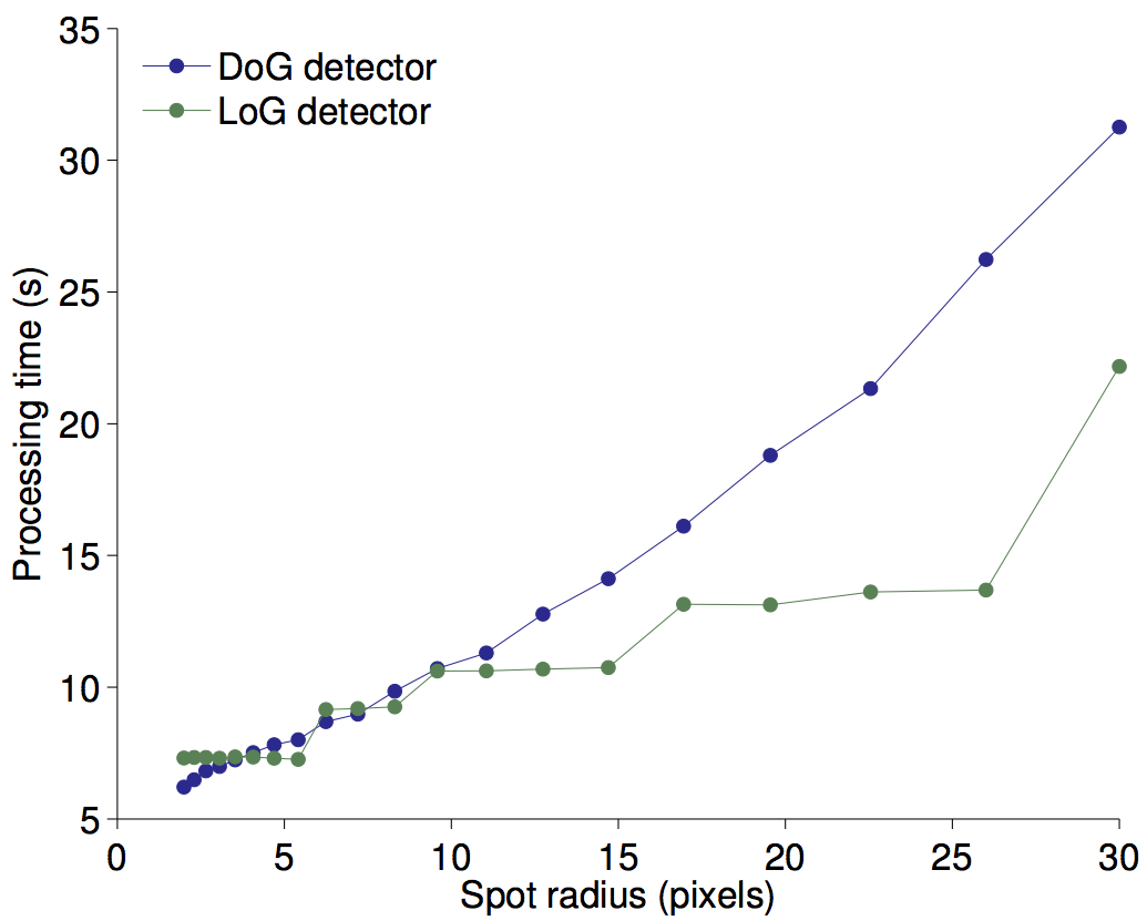
The processing time increases, but this time deviates slightly from linearity in the DoG case. We retrieve the 3D kernel overhead we had for the 3D images.

The LoG performance clearly highlights the 0-padding used because of the Fourier transform: Indeed, the processing time increase in a step-wise manner. We use the Fourier transform to compute the convolution by the LoG kernel. But for the implementation we use, the kernel image (and the source image as well) are padded by 0 until their size reaches a power of 2 (128, 256, 512, etc…). Whenever the required kernel size is smaller than this power of 2, its size is increased to this value. Because ultimately the processing time depends on the number of pixels, we see a constant processing time until the kernel size imposes a larger power of 2.

Choosing between DoG and LoG based on performance

This stepwise evolution makes it slightly harder to choose between LoG and DoG detectors based on performance. As a crude rule of thumb we will remember that

• The LoG detector outperforms the DoG detector in 2D for radiuses larger than 2 pixels.
• The LoG detector outperforms the DoG detector in 3D for radiuses larger than 4 pixels.

References