The content of this page has not been vetted since shifting away from MediaWiki. If you’d like to help, check out the how to help guide!
You will find all functions of the BioVoxxel Toolbox under the icon of the green BioVoxxel cube after selecting BioVoxxel Toolbox from the More Tools Icon (last Icon in the ImageJ/Fiji Icon list with the double arrow).
How to cite
Cite the Toolbox
If you find those functions helpful and use it to generate results you publish, please consider to cite:
![]()

Cite the Figure Tools
The BioVoxxel Figure Tools can be cited separately from the toolbox plugins as follows:
![]()

Extended Particle Analyzer
Purpose: The “Extended Particle Analyzer” is based on the ImageJ “Analyze Particles…” command. It enables the user to further restrict the analysis on particles according to many more parameter spezifications of shape descriptors and angle orientations. Thus, setting minimal and maximal exclusion ranges of different parameters enables to extract particles from a binary image. The output types are the same as for the Analyze › Analyze Particles.
Example: If you want to extract/analyze only particles with a certain Feret’s Angle or exclude elongated structures using the aspect ratio (AR) or circularity you can specify so in the initial dialog box.

How to: Key in minimal and maximal exclusion values connected with a hyphen. You can use integers as well as numbers containing decimal places. “Redirect” redirects the analysis to a grayscale image which enables to analyze skewness, kurtosis as well as the new measure coefficient of variance (cov). The option “Keep borders (correction)” eliminates particles from 2 edges and keeps particles touching the two borders of choice. This corrects the particle count for edge touching particles.
Tipp: use the “Shape Descriptor Maps” macro to figure out possible cut-off value combinations for your analysis which you can then use in the Extended Particle Analyzer.
Shape descriptors which are not available under “Analyze Particles…” in IJ or Fiji so far are:
Extent = [net area of feature] / [bounding rectangle]
Compactness = [sqrt(4 * area / PI)] / [major axis]
Feret’s AR = [maximum caliper diameter] / [minimum caliper diameter]
Coefficient of variance (CoV) = [intensity standard deviation] / [intensity mean]
The new version from 11th February 2018 (included from BioVoxxel_Plugins-2.0.1) on contains 2 checkboxes which enable the choice between pixel and calibrated units in images which are spatially calibrated. The checkbox “Pixel units” is equivalent to the checkbox with the same label in the standard IJ Analyze Particels… function and uses pixels instead of calibrated units to limit the analysis with the respective parameters. The checkbox “output in pixels” gives the option to separately choose if the results table should be in specific units or pixels (depending on the image calibration). Older Macros should still run, while the keyword “pixel” needs to be shifted before the definition of the area parameter.
Form: plugin (recordable, uses smart recording –> records only fields which have been changed by the user while recording. Default entries will not be recorded. It is already sufficient to cut a zero after the comma without changing the actual parameter value to make the recorder recognize that the entry should be recorded!)
Status: Maintenance active
Field-of-view measure correction
Purpose: The macro eliminates all particles in a binary image which touch the edges, then counts the remaining particles and corrects for the counting and the mean area bias due to the edge intersection using the following formula:
count correction factor = (ImgWidth * ImgHeight) / ((ImgWidth-BBWidth) * (ImgHeight-BBHeight))
with “ImgWidth” and “ImgHeight” as the size of the analyzed image and “BBWidth” and “BBHeight” as the bounding box dimensions of each particle. This is recommended as a correction for the bias when measuring features in a field of view because bigger particles are more likely to touch the edges of the field of view and thus their area is are underestimated. This underestimation is proportionate to the particle size. (according to J. Russ, The Image Processing Handbook, 2010, 6th Edition).
How to: only works on individual 8-bit binary images.
Form: macro
Status: maintenance inactive, stable
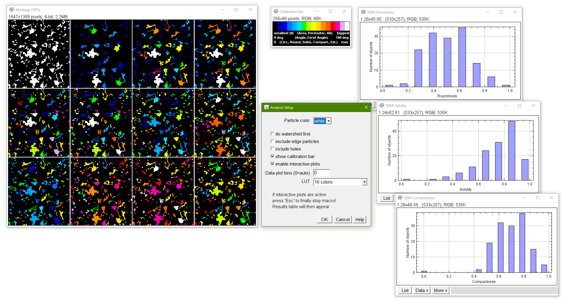
Shape Descriptor Maps
Purpose: Shape descriptors of the particles in an 8-bit binary image will be color coded (smallest to biggest values) and are shown in a stack containing the original image in the first slice and the “shape descriptor maps” in the consecutive ones. The respective shape descriptors are indicated in each slice. A calibration bar (LUT can be selected in the setup) enables easier overview and interpretation. The highest descriptor values can also be displayd as an orientation. When the checkbox “interactive plots” is enabled, the user can simply double-click on one of the slices in the color-coded output stack to receive a distrbution plot of the respective sorted shape descriptor. To finally abort the macro when interactive plots is active “Esc” needs to be pressed.
The distribution might serve to find suitable cut-off sized which then can be used in the Extended Particle Analyzer
This macro helps to visually identify features in images according to their shape properties. Additionally, you can also use the color coded images for consecutive color thresholding after transfering them into RGB mode to extract specific features from the images, according to their coding color.
How to: Select analysis modes and start.
Form: macro
Status: Maintenance active
Binary Feature Extractor
Newer version for 2D and 3D images
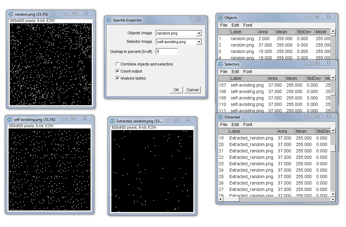
Purpose: The “Feature Extractor” is aimed to select isolate specific features in a binary image by other binary particles as selectors which are located completely inside the features or overlap partially with those. It additionally allows also to get a visual combination of extracted features and selectors (combining those images by using a boolean OR function). The idea for the feature extractor is taken from J. Russ “The Image Processing Handbook” 6th Edition.
Example: A specific nuclear fluorescent staining is thresholded as the selector while the complete cells are thresholded as the features to be extracted.
How to: First, specify the images containing on the one hand the objects to extract and on the other hand the selectors (e.g. marker staining, cell masks) which defines the objects that should be extracted. The plugin then extracts the features which overlap with the selector. The “Overlap in percent” option enables to define a minimal overlap fraction (in percent) of the selector area with the object area (in exactly this sequence). The object is only extracted if the overlap is equal or bigger than the defined minimal overlap. Finally, you can define to show the count of objects, selectors and extracted features as well as display the individual results tables for the three different images (This is equal to run the “Analyze Particles…” on each of the images.
Form: plugin
Status: maintenance active
Speckle Inspector
Newer version for 2D and 3D images
Purpose: The “Speckle Inspector” is able to identify bigger features by the number of containing smaller features/speckles.
How to: In the setup dialog the user can enter the 2 images to be analyzed as well as lower and upper limits of speckle numbers, speckle sizes, object size and object circularity to determine characteristics which include/exclude speckles and features from the analysis according to the entered parameters.
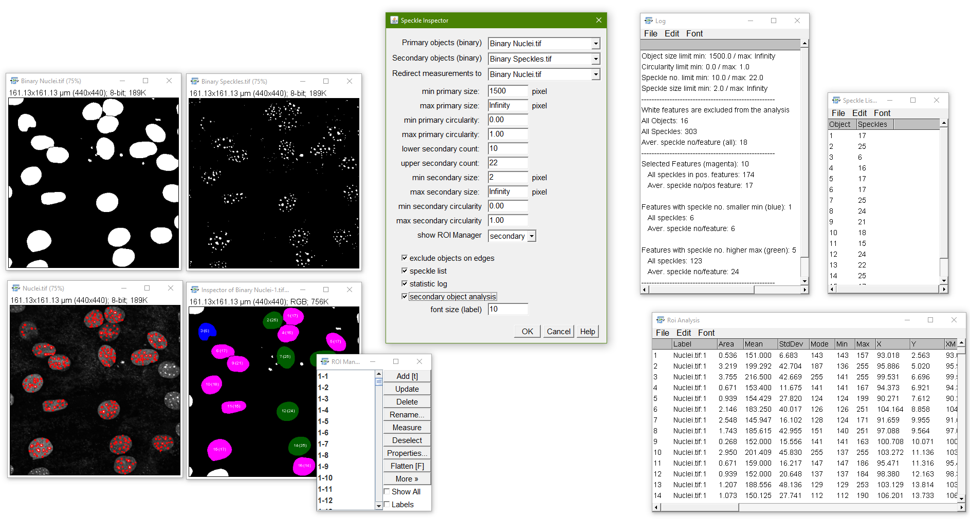
The macro gives different outputs. The optical output is an color-coded image, where positive features (lying inbetween the determined minimum and maximum parameters) are colord in magenta, features containing less than the specified minimum speckle numbers are colored in blue and features containing more than the specified maximum speckle numbers are colored in green. In the same image the features are numbered to identify them in the respective speckle list as well as the ROI manager. Furthermore, they contain the number of “speckles” per feature in brackets. The second output are all feature selection ROIs in the ImageJ/Fiji ROI manager. Moreover a list of all features and respective speckle numbers is given if “show speckle list” was ticked. The “statistics log” window depicts an analysis of the features showing overall numbers of features and speckles as well as the numbers for the features lying below, inbetween, and above the thresholds. You can also choose if you want to see the RoiManager for the objects rois to further analyze the original image. “individual roi analysis” returns a results table which contains the analyzed particles inside each roi (the latter is indicated in the results “Label” column).
New: now the “Speckle Inspector” comes as recordable plugin
Form: plugin
Status: maintenance active
Watershed Irregular Features
The new Label Splitter for 2D and 3D images as alternative Purpose: The standard watershed algorithm in ImageJ is very usefull to separate connected, roughly circular structures. Nevertheless, it gets into trouble while separating irregular (non-ellipsoid like) structures. The Irregular Watershed enables the user to separate also irregular shaped structures to a certain extend.
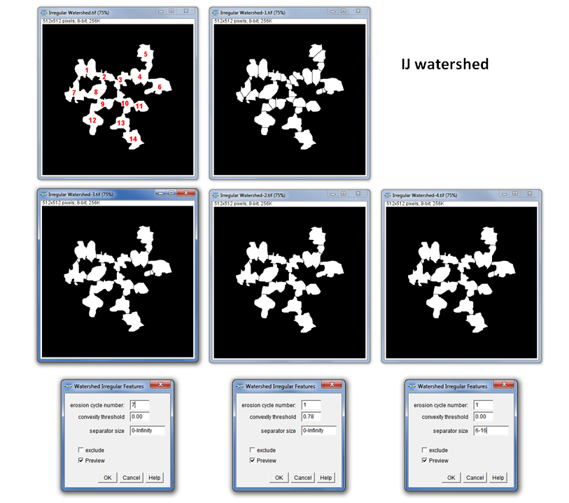
How to: The user needs to specify one of two parameters:
1.) Erosion cycle number: The erosion cycles to be used for the separation algorithm. “0” prevents watershedding. Since increasing numbers use a decreasing size of selector for the separations to be skipped, a too high number might result in unwanted separation in the peripheral regions of the features. Increasing numbers lead to results closer to the standard IJ watershed. The separation only works in the 2D space at the moment and has its limitations when the connecting “bridges” between the features are too broad (as true for the normal watershed algorithm).
2.) Convexity threshold: if this value is above “0” the erosion cycle number is ignored. All objects which have a convexity bigger than the threshold are kept in the image and eroded. If eroded objects coincide with separation lines of the original watershed, those remain in the image and are not used to separate the objects. The sequence of convexity thresholding and consecutive erosion is repeated until there is no object remaining with a convexity above the threshold or the image cannot be eroded any further.
3.) Separator size: the separator size describes the length of the one-pixel line separating connected particles. Thus, the user can specifically choose a size range in which the particle connections should be separated. Additionally, the option “exclude” enables to exclude the specified sizes and separate only connections which are smaller than the lower and bigger than the upper limit.
Form: plugin
Status: maintenance active
Thanks to Thorsten Wagner which provided the ij-blobs library as basis and the idea to integrate convexity as a second parameter to make the function scale invariant and more flexible.
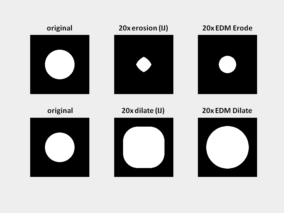
EDM Binary Operations
Purpose: The standard binary erosion and dilation suffers from the artefact that under higher iteration cycles the binary structures get irregularly deformed (see image below, second column). The EDM based methods for erosion and dilation prevent these artifacts. The method is using thresholding on a 8-bit euclidean distance map of the original image to facilitate binary erosion, dilation, opening and closing.
How to: The number of iterations determines how often the chosen function will be applied to the image.
Form: plugin
Status: maintenance active
Auto Binary Masking
Purpose: The macro enables to mask images with their thresholded binary counterparts. Works with 2D images and 3D stacks.
How to: Original and binary mask images need to be identified from the drop-down menu and the user needs to specify if black or white areas in the binary image should be transparent. The output image shows the masked features from the original image.
Form: macro
Status: maintenance inactive, deprecated, stable
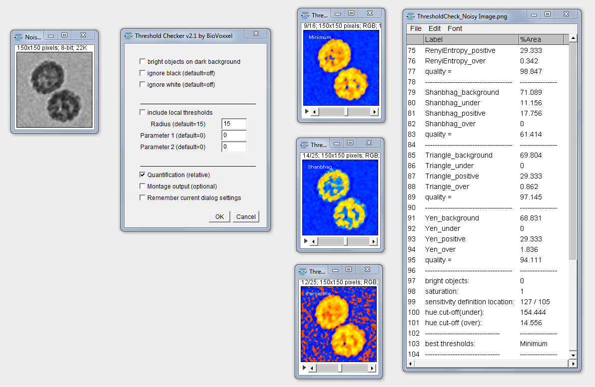
Threshold Check
Newer version for 2D and 3D images
Purpose: The “Threshold Check” should simply provide a help in deciding which of the 16 Auto Threshold and the 9 Auto Local Threshold outputs from the respective plugins results in the potentially best binary image outcome. This is not an absolute measure but should rather assist in the decision for the application of one specific auto threshold algorithm in non-obvious cases. In the new version you can choose additionally to quantify the quality of the thresholding.
How to: The user needs to first select the image the in which the thresholds should be checked (including all the pre-processing you want/need to apply). Be aware to also specify if you are thresholding bright or dark features in the first checkbox! You can also choose to ignore black or white pixels from the threshold calculations (as in the normal AutoThreshold dialog). Furthermore, you can choose to include also the 9 Auto Local Thresholds with the respective parameters (for further reading check out: Auto Local Thresholds. Finally, you can include a quantification of the results and choose if you want to have an overview montage in addition to the normal stack output. Thresholds are indicated in the upper left corner of the images for better identification.
Output interpretation: You will get a stack with each thresholding method represented in a single stack slice. The following colors should help in interpreting the thresholding result:
blue = this is thresholded as background and also represents black or very dark areas in the original image, thus most likely being really background.
cyan = these areas have a certain brightness level in the original image but are not recognized by the respective tresholding algorithm, hence might point out a underestimation of features by the threshold.
orange/yellow = these are features standing out from the background in the original image (orange=medium intensity; yellow=high intensity) which are recognized by the thresholding algorithm as foreground features and thus most likely represent features of interest (depending on the image context and quality).
red/dark orange = these areas have a very low brightness (or are black) in the original image but are thresholded as foreground and therefore most likely represent an overestimation by the threshold.
Caution: Interpretation should be done with care and in context to the original image and imaging settings. This macro is thought to assist in the decision for choosing a good thresholding method. It is no absolute measure for thresholding quality!
Quantification: The Quantification is shown in a results window in %Area. The threshold names are followed by either (under), (positive) or (over). This referres to the following:
- under: the percentage of pixels in comparison to the complete image which seem to be under-thresholded (displayed in cyan)
- positive: the percentage of pixels inside the thresholded region which seem to be well thresholded (displayed in bright orange and yellow)
- over: the percentage (100-positive) of pixels inside the thresholded region which seem to be over-thresholded (displayed in red)
The macro finally suggests thresholds which perform best in respect to the reference point selection. This suggestion depends on the reference point selection and always needs to be compared to the color-coded visual output as well as to the necessities for the following analysis.
Potential issues: If the user does not correctly define if he/she is looking for bright or dark objects the output will be incorrectly determined.
Publication: Qualitative and Quantitative Evaluation of Two New Histogram Limiting Binarization Algorithms. J. Brocher, Int. J. Image Process. 8(2), 2014 pp. 30-48
Filter Check
Purpose: This plugin enables you to test a certain range of radii of a specified image filter in one step. This shoud facilitate a better decision on a suitable filter for your processing purpose. A small hands on descrition is shown as part of the introductory video to basic image processing at the IJ conference in Madison 2015.
How to: Choose a filter method from the drop down menu, key in a starting and an end radius. The image will be filtered in individual integer steps between the start and stop radius and presented in an image stack containing all the filtered images. The filter can also be applied to only a ROI. This is recommended for filters which are cost intensive, like the “Gaussian Weighted Median”. The parameter setting is only needed for the “Bilateral Filter” (range radius) , “Mean Shift Filter” (Color Distance) and the “Linear Kuwahara” (line length).

Form: plugin
Status: maintenance active
Flat-field and Pseudo flat-field correction
Newer version for 2D and 3D images
Purpose: The macro enables to “subtract” background due to inequal lighting from grayscale and true color images. It either uses a previously taken flat-field image (>Flat-field correction) or creates an artificial flat-field image (>Pseudo flat-field correction) from the selected original image. For true color images this is done using the brightness channel of an HSB stack. The original image (brightness channel for true color images) is divided by the flat-field image and the brightness is normalized using the mean intensity of the original image.
How to: You need either choose the two images in the “Flat-field” version or specify a gaussian blurring radius for the “Pseudo flat-field correction” in a way to eliminate specific feature appearance but to keep the difference in shading/lighting. Therefore, rather big radii (sigma) are needed (potentially between 40-150, but this depends on image and feature size).
Remark: The pseudo flat field correction menu command links to the plugin with the same name under Plugins › BioVoxxel (necessary to additionally download from the BioVoxxel update site together with the Toolbox).
Advantage of the Pseudo flat field correction: This is now recordable and works with stacks. Thus, time-lapse movies e.g. from a brightfield microscope can be completely corrected for unequal lighting according to the individual differences in each frame. The blurring is visualized on the currently active frame to be able to sufficiently eliminate structural information.
Convoluted Background Subtraction
Purpose: This tool enables to subtract the background from an image by creating a convoluted copy of the original image and subtracting the filtered image from it. This background subtraction method should facilitate consecutive feature extraction and is not suitable prior to intensity analyses!
How to: The user can choose between Gaussian, Median and Mean convolution filters and key in the respective filter radius (or sigma for the Gaussian Blur). The preview option directly gives a possiblity to compare the results of the background subtraction. The radius for the Gaussian method can be chosen around the biggest feature diameter (as for the rolling ball method). The median and mean methos might need bigger values to avoid elimination of bigger features!
Method: The convoluted images are directly subtracted from the original with exception of the median filtered one. The latter additionally receives a grayscale dilation by application of a maximum filter with the factor (1.5*(radius/10)). This should reduce artifacts around object borders.

Adaptive Filter
(separate plugin under Plugins › BioVoxxel)
Purpose/How to: This filter allows the choice between two basic filter modes (median and mean). The filter Radius defines the size of a square kernel (so actually not really a radius but to keep the entries intuitively similar to other filters in Fiji this label was chosen).
The Shape option enables a basic pre-selection of pixels from the kernel neighborhood to be taken into account for filtering. After pressing ‘Ok’, a checkbox grid will be displayed from which the user can adjust the selected pixels for the final filter according to the filtering needs (e.g. to remove power lines in a photograph).
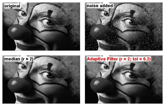
Tolerance sets a threshold which will change intensity values after filtering only for those pixels where the difference to the original intensity is at least as high as the tolerance (0.2 = 20%). This enables to remove extreme outliers from the image while preserving the original pixel values in image areas without such outliers (at least for shot noise).
In the image below the upper pannels show the original photograph and a version with artificial shot noise added. The lower pannels depict the noisy image after a median filter (radius=2) or after the Adaptive Filter (radius = 2 and tolerance set to 0.2) using a circle-like kernel.
Output: The filter will be applied directly on the input image. It is undoable (by pressing [z]).
Limitation: So far, the filter is only applicable on 8-bit and 16-bit single images.
Installation: Part of the BioVoxxel update site in Fiji and can be found under Plugins › BioVoxxel
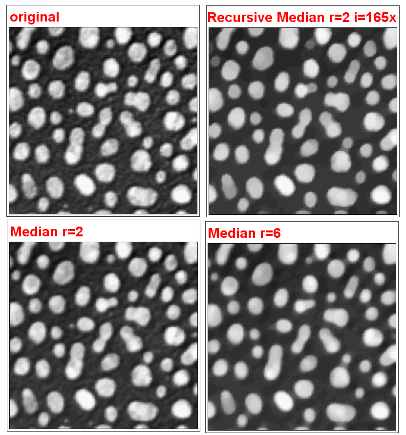
Recursive Filters
Newer version for 2D and 3D images
Purpose: The recursive filters plugin allows to repetitively apply one of the three basic image filters (Gaussian Blur, Mean, Median) with small radii (max = 3) by adjusting the iteration. The previously filtered image will then be taken as basis for the next image filtering
The maximum iteration can be set by the user up to 500 times but will be stopped if two consecutive filtered images do not show any further difference.
Difference of Gaussian and Difference from Median
Purpose: Uses a basic difference of Gaussian method for feature detection and a method which gives the difference between the original and a specified “Median” filter on a copy of the original image.
How to: Difference of Gaussian needs the specification of 2 different Gaussian blurring radii and Difference from Median needs the specification of a Median kernel radius.
Hyperstack Color Coding
Purpose: This macro enables the color coding of the time or volume dimension in stacks and hyperstacks. Multi-channels need to be split up before color coding can be done. The macro is based on the idea of the plugin from Kota Miura and Johannes Schindelin. In contrast to the latter, it keeps the coded stack besides the creation of an additional color-coded z-projection.
How to: Given that you start with a hyperstack, you can choose between time and volume to be color coded. You can choose to create a z-projection by choosing from different projection types (as available in the ImageJ “Z-Project” function). Furthermore, a separated calibration bar can be created which will be horizontal for coded time stacks and vertical for coded volume stacks.
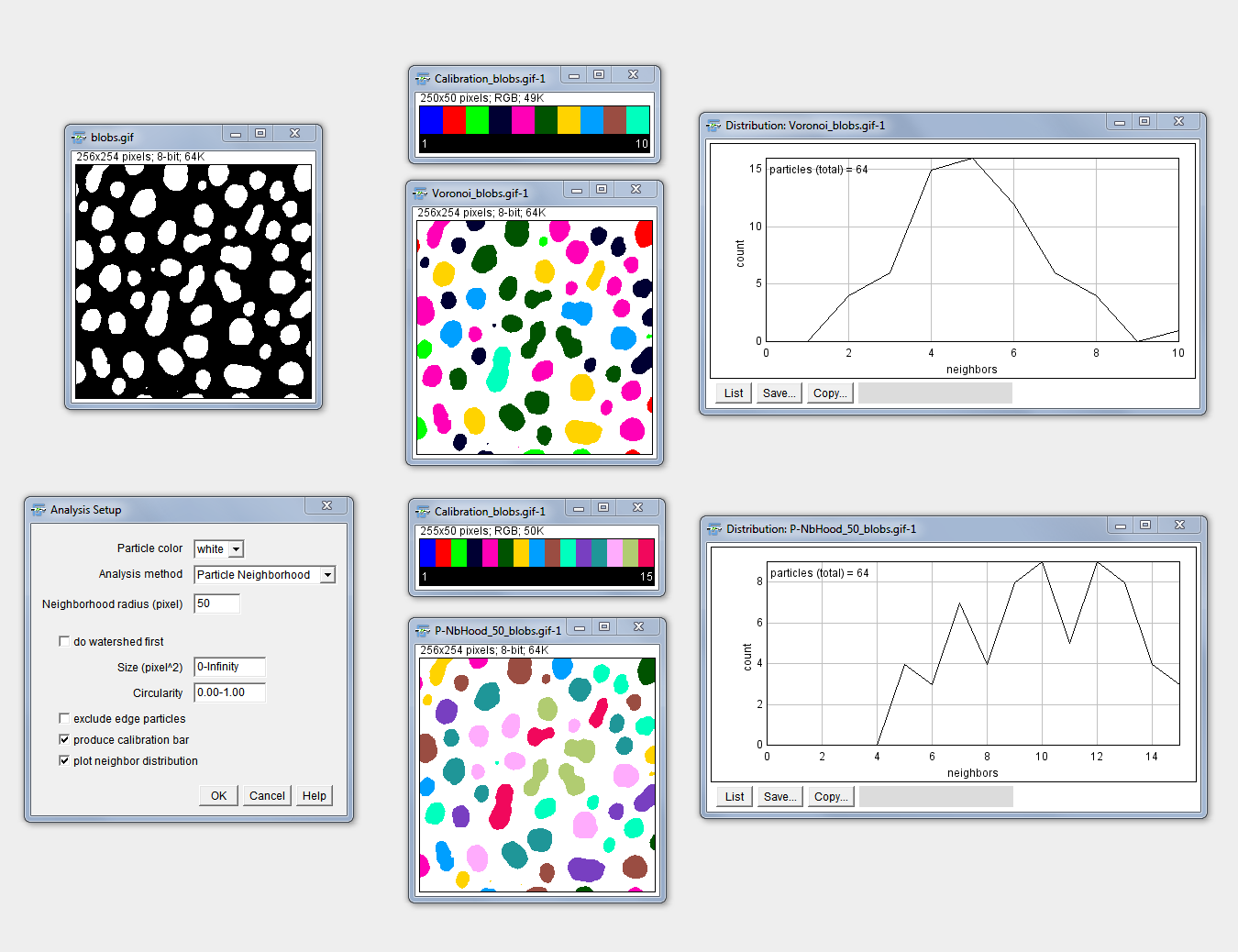
Neighbor Analysis
Purpose: This macro enables the color coding of particles in an 8-bit binary image according to the number of neighbors of each individual particle. Depending on the method chosen, different neighbor particles will be considered during the analysis.
How to: Specify the analysis parameters (same input as for “Analyze Particles…”), choose if you want to include an initial watershed separation of the particles in the starting image and select if you want to display a calibration bar in addition to the analysis output. According to the calibration bar you can interpret the color coding. Mouse hovering over the colored particles enables you to see the respective number of neighbors in the ImageJ/Fiji main window as the number behind “index=”.
Methods: “Voronoi” analyzes the paticles according to the directly correlated voronoi map. “UEP Voronoi” uses the voronoi map from the ultimate eroded points of the particles. This might underestimate the real number of neighbors and is rather suitable for roundish structures. “Centroid Neighborhood” analyzes an area corresponding to a circle with the specified neighborhood radius around the centroid of each particle. “Particle Neighborhood” analyzes also an area around each particle with the specified radius as distance to the particle border.
2D Particle Distribution
(formerly: Distribution Analysis, name changed due to redundency with BoneJ function naming)
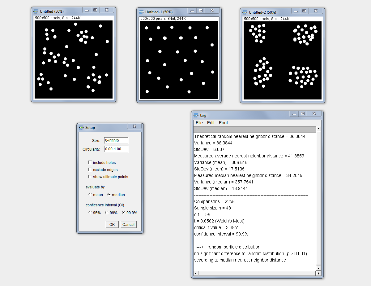
Purpose: This macro statistically determines if particles (according to their ultimate eroded point, UEP) in a 2D image are likely to be randomly distributed, self-avoiding or build clusters.
How to: Starting with a binary image the setup dialog allows similar as the “Analyze Particles” to exclude particles by size and circularity as well as edge touching particles and include holes. The evaluation can be based on the mean nearest neighbor distance or the median nearest neighbor distance. The latter is suitable to better minimize the influence of outliers. Finally, the confidence interval of the statistical evaluation can be chosen between 95%, 99% and 99.9%.
Method: The UEPs of the particles are generated and the nearest neighbor distance is determined for each particle. According to particle number and analyzed area the theoretical nearest neighbor distance is calculated using the formula: 0.5*sqrt(area/n) (according to J. Russ, The Image Processing Handbook, 2010, 6th Edition). This assumption ignores differences in particle size, so far. It is assumed that in the case of normally distributed particles, the mean equals the median. Thus, the method is implemented for the comparison of both, mean and median, from the assumption with the measured values. The measured (mean or median) nearest neighbour distance is statistically compared to the theoretical one. Therefore, first a suitable test method is determined according to the homogeneity of the variance using an F-Test. This finally decides about the use of either a Student’s T-Test or a Welch Test for the final statistical evaluation.
BE AWARE: This tool estimates the type of clustering or exclusion since it does not take non-isotropic shape into account and WORKS ONLY on complete, rectangular images and NOT inside irregular ROIs. This might be changed in future.
SSIDC Cluster Indicator
Meaning: Shape and size invariant DBSCAN based clustering
Pronounce: S-SID C like “acid” C ;-)
Purpose: Indicating clusters of binary image objects after segmentation based on a shape and size invariant density based clustering DBSCAN
Advantage and HowTo: the algorithm detects clusters of any size, shape and number! The user does not need to have any prior knowledge or estimation of a number of clusters (as for e.g. k-means). The only input needed is the isotropic distance (in pixel) the user wants (epsilon in DBSCAN) to check around each object and a desired minimum density (number of objects inside the given distance). The algorithm reaches out equidistantly from the object shape. Therefore, amorphous shapes of particles do not matter. Furthermore, the size is not relevant, since the distance is taken from the outside of the object. If size and shape should be ignored, the plugin can be run on the thresholded (min=1 max=255) ultimate points of the binary objects Process › Binary › Ultimate Points Clusters are also detected in an overlapping but still separate manner if some objects might belong to several clusters but do not belong to their core points.
Output: The output is on purpose very sparse and gives only the ImageJ ROI Manager. From there cluster numbers and individual amount of objects per cluster can easily be analyzed e.g. using a macro on the ROI manager and the corresponding image
Application: The algorithm was already successfully applied in the quantification of clusters from different cell populations in microscopic mouse retina samples [Link once the manuscript is accepted and published]
Limitation: works on 2D binary images only and does not detect clusters inside other clusters
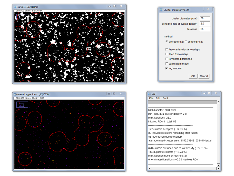
Cluster Indicator
(depricated)
Purpose: The “Cluster Indicator” is thought to detect local particle clusters in a binary image. Different particle sizes can be taken into account.
How To: Choose a cluster detector size as a circle radius in pixels. The density (as a x-fold value) enables to adjust the sensitivity because found clusters are only accepted as a cluster when their density of neighbor distances is at least x-fold of the average neighbor distance in the complete image. Two possible methods can be chosen:
1.) “average NND” uses the inverted 32-bit Voronoi image as measure of the between-particle (border-to-border) distances to all of their neighbors. This accounts for differences in particle size as well as shape. The average neighbor distance is taken to intensity code the centroid point in the evaluation image.
2.) “centroid NND” uses the ultimate eroded point map and intensity codes the points according to their nearest neighbor distance. This method is faster especially for big images with many particles but neglects differences in particle size and shape. Therefore, might only be applicable if all particles are equal in size and shape.
Each individual cluster finding process is aborted if a local cluster was not found after the specified number of maximal iterations. Those aborted clusters can be shown as blue ROIs in the image if desired (see checkbox).
Clusters overlapping (at least 1 pixel) can also be fused to one cluster if specified so by the respective checkbox.
Consider that the detector size as well as density settings influence if a cluster is found and finally accepted as a cluster. This on the one hand leads to a certain bias but should enable the user to search for clusters of different sizes and densities.
Method: Circle ROIs of the specified size are initially distributed with sufficient overlap to cover the complete image. The cluster finding process is done according to the mean shift method towards the center of mass of clusters. The latter is influenced by particle number, size and neighbor distance.
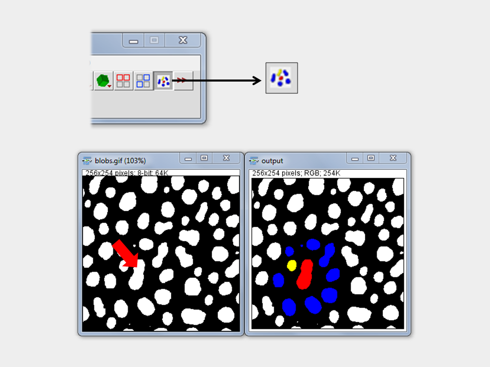
Nearest Neighbor Indicator (Separate Tool)
Purpose/How to: This tool enables the user to click in any feature in a binary image to identify all neigbors and the nearest neighbor of this feature. Therefore, the tool needs to be activated. Then any click will lead to a new calculation of the neighbors depending on the location clicked on.
Output: A copy of the original image is created with the particle of interest (POI) in red, neighbors in blue and the nearest neighbor in yellow. If more then one neighbor has the same distance to the POI all neighbors with that distance will be indicated in yellow.
Method: As measure for the distance between the particles the minimum separation distance is taken by analysis of the intensity coded Voronoi cell algorithm of ImageJ. The lowest non-background intensity is used to indicate the nearest neighbor.
Gaussian weighted Median filter
(separate plugin under Plugins › BioVoxxel)
Purpose/How to: This filter is basically a normal median filter (as in ImageJ/Fiji) but with a weighted filter matrix. The radius is given in pixels. The weight is determined automatically by a 2D gaussian function (approximated to integer values) over the size of the filter grid. Thus, pixel closer to the filter center get a higher weight compared to more distant ones. This reduces the intensity homogenizing effect from a normal median filter but increases the edge-perservation of features.
Output: The filter will be applied directly on the input image. It is undoable (by pressing [z]) and will be recorded by the macro recorder.
Limitation: So far, the filter is only applicable on 8-bit and 16-bit single images.
Enhance True Color Contrast
(separate plugin under Plugins › BioVoxxel)
Purpose: This image filter enhances the contrast of true color images similar to the method Enhance Contrast in Fiji. If the latter would be applied to true color images this leads to a change in color values and saturation. This unwanted effects are eliminated by the recordable “Enhance True Color Contrast” plugin. It preserves color tone and saturation while enhancing the contrast in the brightness channel of the HSB color space. This is done using high precision float value calculation and not by a simple conversion o fthe image to HSB color space as available in ImageJ/Fiji. The latter would lead to a loss in quality since due to conversion and back-conversion to RGB.
How to: The user can key in a percentage of saturated pixels as in the “Enhance Contrast” function and has a preview option.
Mode and Differential Limited Mean Binarization
(separate plugin under Plugins › BioVoxxel)
Purpose: The mode-limited mean (MoLiM) and the differential-limited mean (DiLiM) are two binarization algorithms which initially limit the image histogram according to its mode value (MoLiM) or its mode, an initial mean or the median (DiLiM). A more detailed description can be found under:
Qualitative and Quantitative Evaluation of Two New Histogram Limiting Binarization Algorithms. J. Brocher, Int. J. Image Process. 8(2), 2014 pp. 30-48
How To: the user can choose to use the differential threshold determination or the forced mode-limited method if “differential limitation” is off. The algorithm assumes that the features occupy less than 50% of the images space independent if they are bright on a dark background or vice versa. For the opposite case one would need to invert the final output image. The limitation step eliminates all intensity information in the histogram up to the limit (mode, mean or median) and calculates a new mean value which is taken as final threshold. “Force to smaller partition” enables to extract the pixels which occupy rather the smaller histogram partition besides the limit.
Download: Part of the BioVoxxel update site in Fiji and can be found under Plugins › BioVoxxel
Leica ROI Reader
The Reader can open and read Leica ROI files saved by the LAS software (tested only for LAS AF). and add them to the ImageJ ROI Manager.
License
The BioVoxxel Toolbox project runs under the BSD-3 License