AplimTools

The content of this page has not been vetted since shifting away from MediaWiki. If you’d like to help, check out the how to help guide!

AplimTools is a set of image processing tools for plants magnetic resonance analysis. These tools are developed in the context of the Aplim project (see the project official page ). Main features :

T1/T2/M0 maps computation from spin echo sequences (multiple TR and/or TE)
Time-lapse exploration of T1/T2/M0 parameters in interest areas

full-1 — Time-lapse exploration of parameters in a plant under drought stress

Installation

In order to install AplimTools on your computer, please follow these simple steps:

1. (if needed) Download and install Fiji from https://fiji.sc/ ; start Fiji, and let it automatically update. Then restart Fiji.

2. Open Fiji, run the Update manager Help › Update. Click on “OK” to close the first popup windows, then click on the button Manage update sites….

3. In this list, activate ImageJ-ITK by checking the corresponding checkboxes. Don’t close the window, or reopen it you read this to late.

4. Add the Fijiyama repository (by clicking on the button Add update site, and filling the fields : name = “/plugins/fijiyama”, site = https://sites.imagej.net/Fijiyama), then check the associated checkbox. Don’t close the window, or reopen it you read this to late.

5. Add the AplimTools repository (by clicking on the button Add update site, and filling the fields : name = “/plugins/aplimtools”, site = https://sites.imagej.net/AplimTools), then check the associated checkbox. Now you can click on Close.

6. Restart Fiji: a new AplimTools entry should be available in the menu Plugins › Analyze. If not, go back to the Update Manager, and check that the repositories ImageJ-ITK, Fijiyama, and AplimTools are correctly selected.

Aplim T1/T2/M0 maps importer

The science behind

This plugin compute M0, T1 and T2 maps pixelwise from a given set of spin-echo sequences, acquired with different repetition times and/or different echo times.

First a 3d registration is computed to align precisely the successive images, using libraries of the [Fijiyama] plugin. Then the rice noise level is estimated, and the M0, T1 and T2 parameters are estimated, fitting mono or bi-exponential curves, corrected with the measured rice noise (reference : https://onlinelibrary.wiley.com/doi/full/10.1002/mrm.22178 [Raya et al., 2010].

Preparing your data

This plugin needs properly formatted dataset, a SL_RAW directory (whatever be its exact name) with exported data in it. To construct it, use the BionanoNMRI scripts, with the processing.bnp parameters set to :

Create RAW DICOM set to yes.
Create CLEAN DICOM set to no.
Create MASK DICOM set to no.

and using a listSer.ser file including all the interesting data for the T1 and T2 sequences.

Running the plugin

The plugin ask for the SL_RAW directory (see above), then an output directory to write results, before asking some questions about the computation you want:

Register data ? Answer No means you are really confident about the exact positioning of the object. You should answer Yes
Register T1 and T2 ? When providing T1 and T2 sequence, to get proper results and analyze, you should answer Yes, in order all the exported results (T2, M0 and T1 maps being aligned)
Register Manually ? Answer Yes if the data are really misaligned (angle > 30 degrees, translation > the object half-size)
Register Dense ? Answer Yes if the object could undergo some deformations during experiments (growing, stretching in the antenna, drying…)
Register successive T1 ? Answer No means you are really confident about the exact positioning of the object. You should answer Yes
Use T2 in T1 sequence ? You should.

After all these questions, the plugin run the registrations, and compute the maps. It can last a while (typically 1 min. for a 512 x 512 slice).

Finally, the maps are concatenated in an hyperimage, saved in your output directory

Exploring the results

The output image is a 4D MR hyperimage. The “channels” slicer helps you to explore the 4th dimension, that is the images computed, and the input spin echo images. In detail :

Channels 1,2 3 are respectively the M0 map, T1 map, T2 map (see this information in the slice title, just upside the image pixels)
Channels 4,5, ….. NR-3 are the successive NR repetition times of the “T1 sequence”, in increasing order.
Channels NR-2,….. NR-2+NE are the successive NE echo times of the “T2 sequence”, in increasing order.

Unit for the channels 2 and 3 are milliseconds, what mean you can use it like it, without any additional conversion.
For time-lapse experiments, one can compute such a 4D MR hyperimage at successive timepoints, and register and combine them in a 5D MR hyperimage (the same, with an additional slicer to walk through time). Registration and data combining can be done using the plugin [Fijiyama], using the Series registration mode .

Aplim T1/T2/M0 curves explorer

Exploring relaxation curves

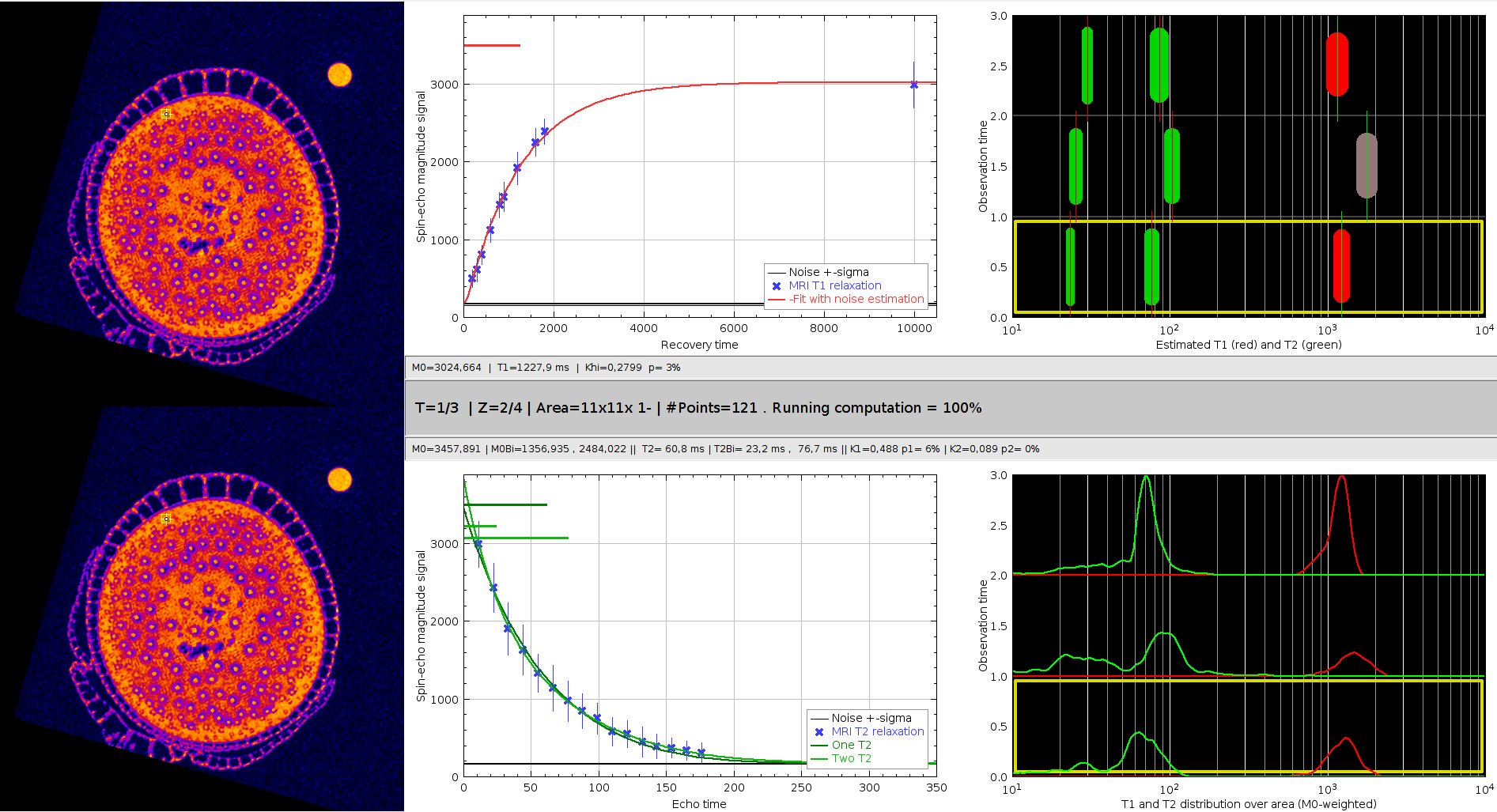
This plugin helps exploring the relaxation curves on a point, the neighbourhood of a point, or a user-defined roi, using non-linear fit (as above). The visualization of these curves (middle panels) is enriched by semi-log graphs of the T1 and T2 values (right-top panel), and a distribution of these values in the selected area (right-bottom panel). This explorer can open time-lapse 5D hyperimages, to give insight of the evolution of these parameters along the experiment. The explorer display informations through 6 panels :

Panels details

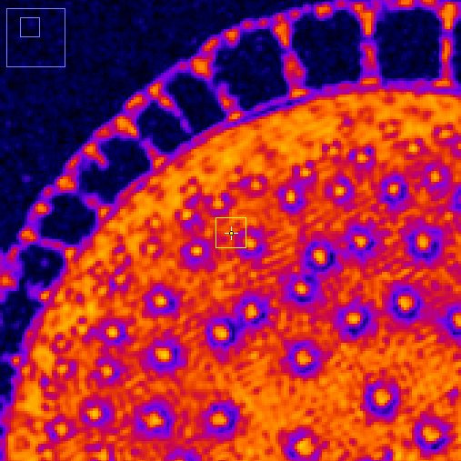
Left panels: spin echo images from T1 (top) and T2 (bottom) sequences. The yellow square shows the interest area where the tissue parameters are estimated. Its size and position can be modified dynamically.

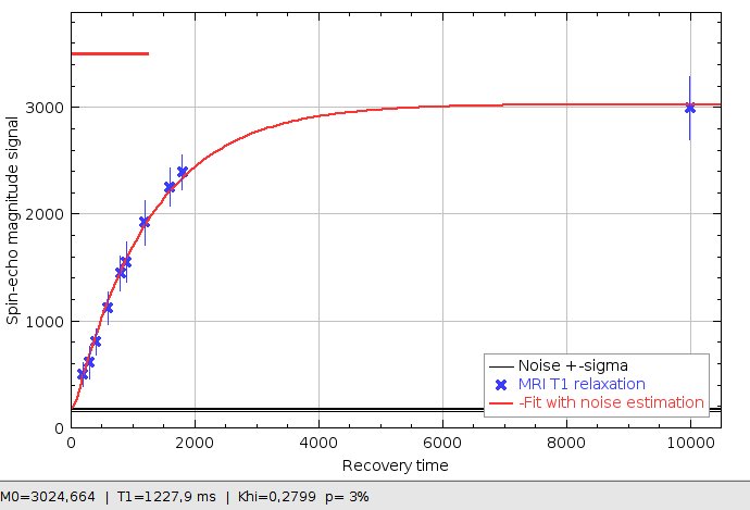
T1 relaxation curve (red) estimated from MRI data (blue crosses), given the measured noise level (black)

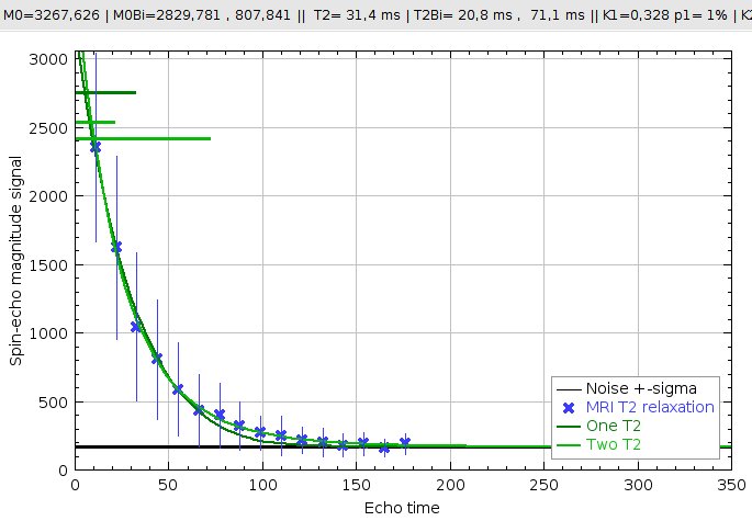
T2 relaxation curve (dark green=mono-exponential, light green=bi-exponential) estimated from MRI data (blue crosses). The blue crosses display the mean MR value over all the pixels in the interest area (the yellow square), and the std within these data is displayed as a vertical blue bar. The measured noise level used for noise-corrected estimation is displayed as a black line.

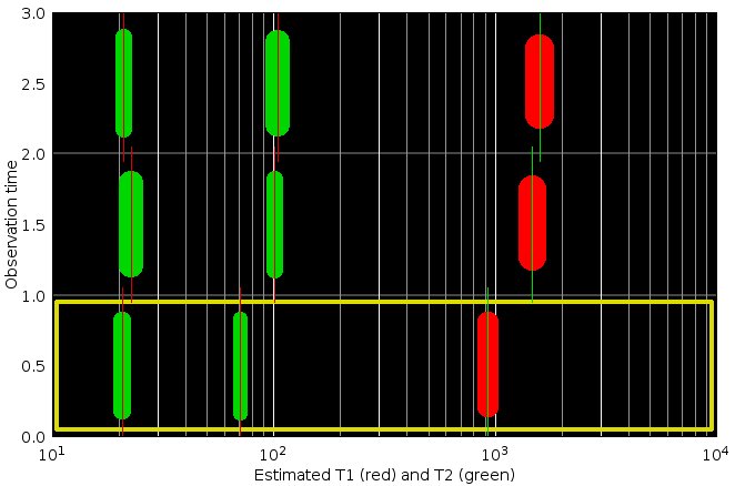
Values of T1 (red) and T2 (green) estimated from the mean values (blue crosses on the curves panel). Marker thickness are proportional to the relative proton density. The three graphs (from bottom to top) shows the values in this area for the three successive timepoints of the 5D MR Hyperimage.

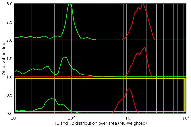
Distribution of the T1 and T2 values estimated from each individual pixel of the current region of interest.

References

- José G. Raya, Olaf Dietrich, Annie Horng, Jürgen Weber, Maximilian F. Reiser, Christian Glaser, 2010. « T2 measurement in articular cartilage: Impact of the fitting method on accuracy and precision at low SNR ». Magnetic Resonance in Medicine 63:181–193 (2010)
Software dependencies acknowledgements
- Johannes Schindelin et al for Fiji (Schindelin et al., 2012)
- Karl Schmidt and Curtis Rueden for tips seen in the MRI Analysis Calculator and in the CurveFitters
License
This program is an open-source free software: it can be redistributed and/or modified under the terms of the GNU General Public License as published by the Free Software Foundation (http://www.gnu.org/licenses/gpl.txt).
This program is distributed in the hope that it will be useful, but WITHOUT ANY WARRANTY; without even the implied warranty of MERCHANTABILITY or FITNESS FOR A PARTICULAR PURPOSE. See the GNU General Public License for more details.