Introduction
This tutorial show how to manually edit, correct and create spots and tracks in TrackMate. You might want to use manual editing to correct mistakes of automated segmenting or tracking, to do a full manual annotation of a dataset, or to create a “ground-truth” data.
Manual annotation is seldom the most adequate alternative: depending on the size of the target data, it can take an important amount of time and energy, is not objective, and is not reproducible. But sometimes you have to bite the bullet, whether because a segmenter does not exist for your kind of images, or because it is quicker to manually correct error than to come with the ultimate, flawless algorithm.
Also, tracking is difficult in bio-imaging: images have by construction often a very low SNR, and there is a very wide range of variability amongst experiment types. TrackMate includes generic tracking and segmentation algorithms, and therefore does not exploit the specificity of each problem. It is likely that there are going to be some defects on the difficult use cases you will use it on, and these defects should not stop your science. So there should be a way to manually correct and edit the tracking results. We tried to make it as convenient, easy and quick as possible in TrackMate, should your science requires it.
It is a good idea to be already familiar with the automated segmentation in TrackMate, following the Getting started with TrackMate tutorial. Here, we will use an incorrect automated segmentation result, and correct it manually. It is perfectly possible to skip the automated part and to do the whole process manually.
The test image: Development of a C.elegans embryo
Download the target image here: Celegans-5pc-17timepoints.tif (94 MB).
Open it in Fiji. You will get a stack, made of 41 Z-slices over 17 time-points, each image being 240 x 295. As you can see in Image › Properties (⌃ Ctrl + ⇧ Shift + P), it has a spatial and temporal calibration.
The context if the following: We used a C.elegans strain named AZ212 that has its histone H2B coupled to the eGFP. The nuclei can therefore be seen in the 488 nm excitation fluorescence channel. The movie started just after the first cell division, so you can see on the first frame two blob-like spots in the center of the egg. On the top-right part of the egg, there is also two smaller spots that are the polar bodies. One will remain at a fixed place, the other one will be pushed around as the cells divide. The movie has 17 time-points that span the first 34 minutes of the C.elegans embryo development.
We were trying to assess the impact of phototoxicity on development in this movie. We used a rather strong laser power, which explains the relatively good quality of the image, and the fact that this egg’s development is slowed down compared to a classical development at 21°C. On this movie, I manually erased another egg that was lying on the top left-corner of the image, which makes it suitable only for educational purposes.
We want to reconstruct the cell lineage from this movie. Ideally, we will end up in having four tracks: two for the the two cells present on the first frame, and two for the polar bodies. The cell tracks will be branching, following cell division.
This tutorial uses the following strategy: we will use an inadequate set of segmentation parameters to simulate defects in segmentation. Then we will use a tracking algorithm that does not take into account the possibility for a cell to divide, and will not use the spot feature to make linking robust, thus generating linking defects. Finally, we will learn how to correct these defects manually.
Doing a fast but very bad segmentation
Launch TrackMate (Plugins › Tracking › TrackMate) and select the C.elegans stack as a target. Check on the first panel that all the spatial calibration is OK. The pixel size is about 200 nm in XY, 1 μm in Z, and each frame is separated by 2 minutes.
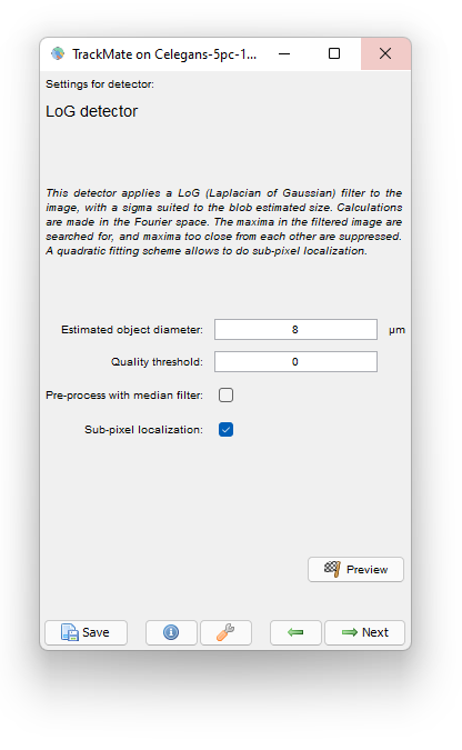
Select the LoG detector. This choice actually makes sense: the nuclei are about 8 μm in diameter, and with a sampling of 200 nm, that makes 40 pixels wide nuclei. It is already advantageous to use the LoG segmenter above 15 pixels as we observed it is faster than its DoG counterpart for large objects.
The segmentation should take you no more than a minute, even on a standard machine, a considerable improvement over a standard segmenter. But at what cost!

On the Initial thresholding panel, we see that it is easy to separate spurious spots using the Quality feature only. There is a big and sharp peak at the left of the histogram. By moving the slider around you can get the remaining number of spot after filtering. If we put the threshold around 40, just above the first sharp peak, we see that we are left with about 177 spots. Now: We have 17 time-points, each of them containing at most 4 cells and two polar bodies (check the raw movie). So 177 remaining spots seems to be above the number of spots we should get in an ideal case. We will have to filter some of them later.
On the Spot filters panel, the results of the detection will appear. It is likely that our results are the same if you used the same numerical values as above. And you can see that there are still a lot of spurious spots amongst the remaining 177. We were not stringent enough when we selected the initial threshold.
Anyway, let’s correct it now. Just add a filter on Quality, and take a value of 200; 74spots should remain, and the spurious ones should disappear.
Almost all polar bodies are incorrectly detected, and the localization of cells is bad. These are expected defects given our choice of detection algorithm and the parameters we have used. Here, the results are not so bad, unfortunately for this tutorial. We could fix them right now, before tracking. You can actually edit the results any time after the first panel of TrackMate. But let us exploit these defects for our training purpose, by having them generating additional linking defects.

Generating irrelevant tracks
Normally, TrackMate can robustly handles track splitting events, representing e.g. cell division. Though this happens in this movie, we choose to dismiss this possibility in the automated tracking part.
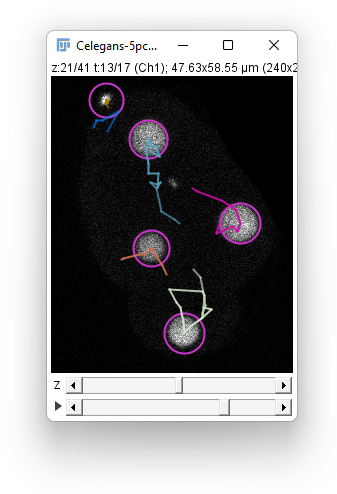
In the Tracker choice panel, select the Simple LAP tracker. Leave the default values for the parameters (15 μm for the 2 distances and a frame gap of 2) , and press Next. You should end up in having something similar to the image above.
A quick assertion shows that for nuclei, the individual track branches are not so bad. Each of the retained spot could use some fine tuning, but the tracks are not completely pathological, disregarding the fact that splitting events are missed. The polar bodies tracking results are hopeless.
This is what we will now manually correct.
Launching TrackScheme
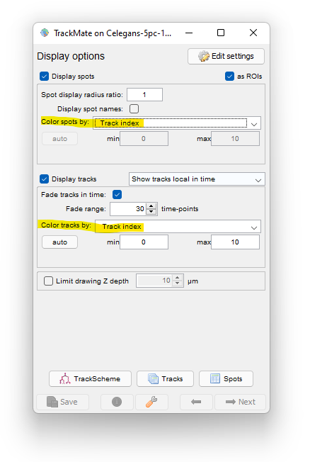
Move to the Display options panel, skipping the track filtering part.
First let’s edit the display options so that the spots are colored by their track index.
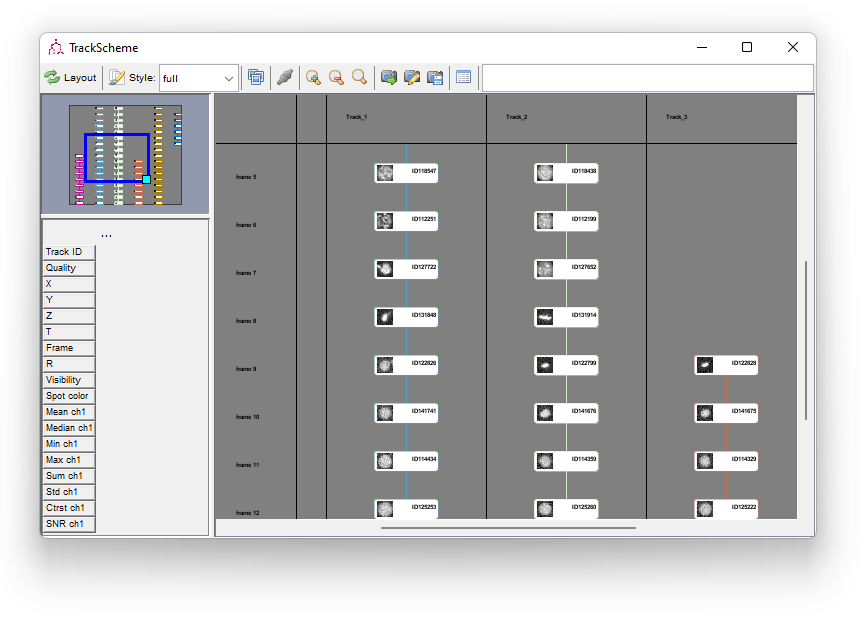
TrackScheme is a TrackMate tool for the visualization and editing of tracks. It displays a kind of “track map”, where a track is laid on a pane, arranged vertically over time, as a Parisian subway train map. Tracks are displayed hierarchically, discarding the spatial location of each spot. Each spot is laid out going through time from top to bottom. It is a great tool particularly to study and edit lineages.
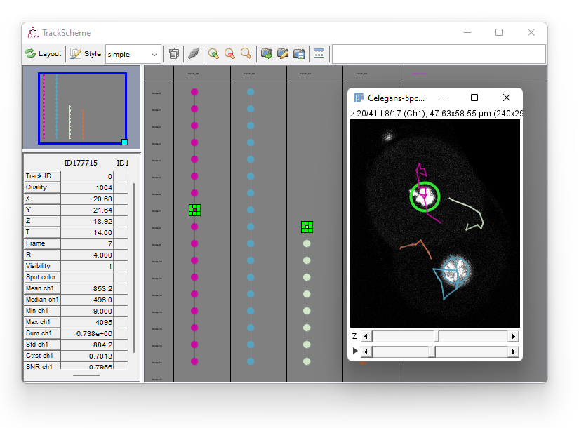
TrackScheme also allows manually editing the tracks. Press the TrackScheme button on the last panel. By default, the tracks are displayed as colored circles joined by lines. Each circle represent a spot, and the lines represent a link connecting two dots. The selection in TrackScheme is share across TrackMate, so if you select one circle, it will be highlighted in the HyperStack viewer as well (circled in green).
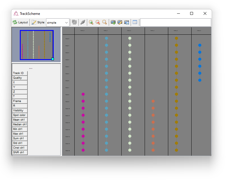
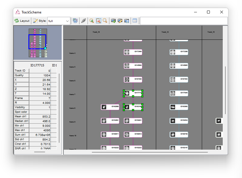
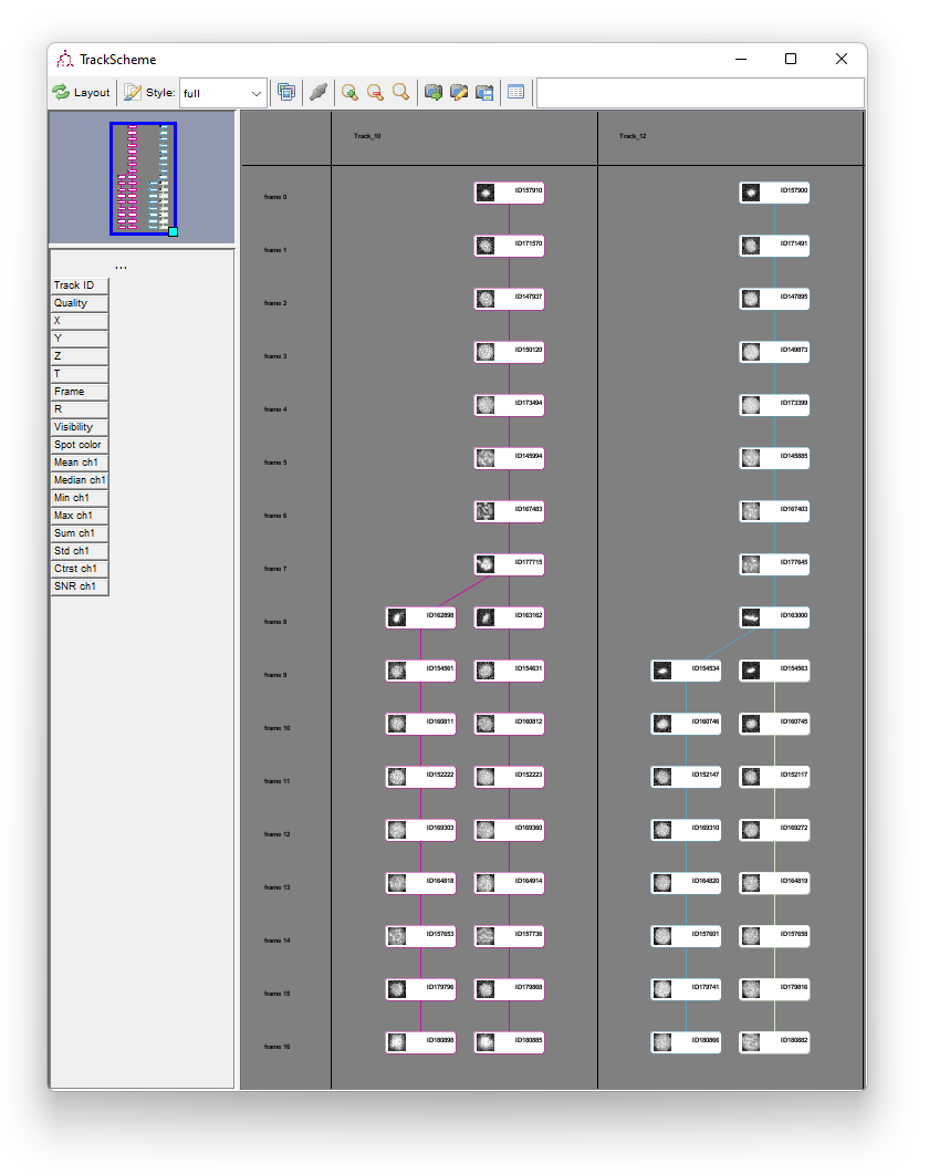
TrackScheme launches with a simple style: each spot is represented with a circle. You can get more information by changing the style. Next to the Style button in the TrackScheme toolbar, there is combo-box ini which you can select either simple or full. Select full. Each spot is now represented by a rounded rectangle, with the default name printed on the right. Go back in the TrackScheme toolbar. Next to the style combo-box, there is greyed-out button showing 3 pictures. Press it; after some time, each spot in TrackScheme will contain a thumbnail of the spot taken in the raw image. This is very handy to quickly detect detection problems.
TrackScheme in a nutshell
You can do quite some things using TrackScheme, notably track analysis. This is not the ofcus of this tutorial, we will simply be focusing on the track editing features. However, here is a brief description of what the toolbar buttons do.
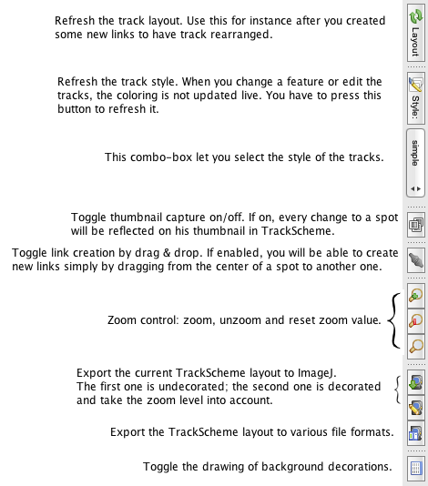
We will be mainly using the Redo layout and button.
Getting rid of bad tracks
We will first start by removing all the bad spots and tracks. We decide not to keep the tracks generated by the polar bodies, and only to keep the tracks that follow the 2 nuclei.
- Move to the Track_4 column in TrackScheme. You can see that it is following the static polar body.
- We wish to select it at once. There is two way you can do it:
- Draw a selection rectangle around the whole track representation.
- Select one spot or link in the track.
 Right Click anywhere on TrackScheme: a menu appears, in which you will find Select whole track.
- Notice in the displayer that the selected track appear with a green and thick line, so as to highlight it.
- To delete all of it, simply press the ⌦ Delete key in TrackScheme, or use the right-click menu to do so.
Do the same for Track_5, since we do not want to include polar bodies in the subsequent analysis.
Press the Redo layout button when you are done. There should be four tracks remaining. Notice that their color changed as you deleted some of them. Their color is re-adjusted every time the track number changes.
Spot editing with the HyperStack Displayer
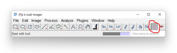
We now wish to correct for segmentation mistakes, that caused some nuclei to be missed. Creating new spots is made directly in the HyperStack displayer. First, make sure the TrackMate tool (represented by a purple track) is selected in the ImageJ toolbar, as pictured below:
The HyperStack displayer let you edit spots combining the mouse and keyboard. I have found using the mouse clicks sub-optimal and painful for the carpal bones when editing a lot of spots. Using a combination of the mouse and keyboard proved to be more efficient.
This page contains a summary of the keyboard shortcuts we use here.
Moving an existing spot
- Position the mouse over the target spot (you do not need to select it).
- Hold the ␣ Space key.
- Move the mouse around. The target spot follows the mouse location until you release the mouse key.
Creating a new spot
- Position the mouse anywhere on the image.
- Press the A key.
- A new spot is added at the mouse location.
By default, the new spot has the radius of the last spot edited.
Deleting an existing spot
- Position the mouse over the target spot.
- Press the D key.
- The target spot is deleted
Changing the radius of a spot
- Position the mouse over the target spot.
- Press the E key to increase its radius, Q to diminish it.
- ⇧ Shift + Q and ⇧ Shift + E change the radius by a bigger amount.
Adding missed spots
You now have the tools to correct the mistakes our crude detection made. Unfortunately for is exercise, there isn’t a missed spot with the settings we used. So we will simulate missing spots by deleting the last spots of the 4 tracks in the last time-point. In the image window, move to the last time-point and select a Z-slice in which the 4 spots are visible (drawn as circles). Put the mouse inside each spot and press the D key to delete them. These deletion can be seen in the TrackScheme window as well.
Now let’s add the spots back. Position the mouse and the Z-slice where cell is and press the A key. A new spot appear with a default radius. Note that its color is grey. We chose to color spots by their track index and this new spot does not belong to a track yet.
Edit its radius with E and Q so that it matches the cell radius. You might have to move the spot to center it (press and hold ␣ Space as you move the mouse).
Notice also that when you add spots, they also appear in the TrackScheme window as a grey cells, on the far right in a lane without track number (under the column Unlaid spots). As long as you do not incorporate them in a track, they will remain there.
You should end up in having a corrected segmentation, where every nuclei correspond to one spot in TrackMate, and it at the right location. However the 4 new spots are not linked to a track yet, and the TrackScheme window should resemble this:

Time yourself doing so, so that you learn how much you have to invest on manually correcting segmentation results, and decide if it is acceptable.
Editing tracks: creating links
Now we want to connect the lonesome spots to the track they belong to. This is all about creating links, and there are two ways to do that.
By drag & drop
You can create a link between two cells in TrackScheme simply by enabling the linking button on the TrackScheme toolbar, and dragging a line between the source cell and the target cell.
This is pictured below, where the fore-to-last cell of the track 4 is connected to the new spot. For visibility, I brought on this screenshot the target cell closer to the lane of the track 4. You can normally find it either on the far right of the panel.
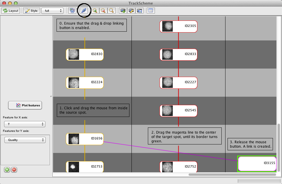
Press the Redo layout button to see the arranged result. The spots is now incorporated in the right track. Note that the color of the spots you incorporated in the tracks has not changed yet. The colors in TrackScheme are updated only when you press the Style button.
Using selection and right-click menu
The cell in TrackScheme cannot be easily moved. Also it can be difficult knowing what spot in TrackScheme corresponds to what spot in the image when you have many. When the source and target cells are far away, it might be better to use another way to create links. We do this using the shared selection.
To illustrate this we will now merge the two daughter branches to their mother after cell division.
In TrackScheme, find the first spot of the top-right track, in frame 9. When you click on the corresponding cell in TrackScheme, it gets highlighted in green. In the HyperStack viewer, the displayed slice and time points are changed to display the spot, also highlighted in green.
We want to link this cell to the mother cell in the top-left track, frame 8, just before it divided. To do so,
- In the HyperStack displayer, move to the frame 8
- Hold the ⇧ Shift key
- Click on the mother cell
It gets highlighted in the displayer, and in TrackScheme as well. You now have two cells in the selection.
To create a link between the two,
- Right Click anywhere in TrackScheme
- In the menu that pops-up, select Link 2 spots.
The newly created link is displayed in magenta. Note that the track arrangement is not changed; you need to press the Redo layout button to rearrange the tracks.
After doing so, you should now see a branching track, as picture below. Notice that the track colors are out of sync. The colors are not automatically updated when changing a track layout. You have to click the Style button in the TrackScheme toolbar to do so. Do so.
Creating several links at once
Using ⇧ Shift +  Left Click, we can put several cells in the selection, and create the links between each pair. We don’t have the need for it, but this is a good way to create a single track from several solitary spots: Just select them all (dragging a selection box or ⇧ Shift + Left Click) and select the Link N spots menu item.
Editing tracks: deleting links
We do not have much to say here. The tracks we generated had missing links, but no spurious ones. So we do not need to remove any. But here is how to do it:
In TrackScheme, select the target link by clicking on it; it gets highlighted in the displayer as well. Press the ⌦ Delete key to remove it.
Removing a link often splits a track in 2 new tracks. To have them properly re-arranged, press the Redo layout button.
Wrapping up
Plus or minus the localization errors and some incorrect cell radii, you now have the full lineage in 3D of this short movie. This concludes this tutorial on manual editing in TrackMate. Here is a picture of the final results:
Jean-Yves Tinevez - Jan 2022