TrackMate-ExTrack: diffusion and binding kinetics in live cells.

TrackMate-ExTrack is a TrackMate action that contains a port of the Python analysis tool ExTrack to Java and TrackMate. The paper that describes the science behind this tool is here:

doi:10.1083/jcb.202208059

Please cite it if ExTrack is useful for your research.

The Python version of ExTrack, which should be considered the nominal and prime source, can be found on its GitHub repo. This page solely documents the TrackMate port.

ExTrack analysis in TrackMate.

ExTrack performs track analysis and can determine whether a particle is undergoing diffusive motion or is bound and appear as stuck. Importantly, ExTrack can resolve the transitions from one state to another for a single particle. It is built to be robust against noisy trajectories and offers an excellent accuracy even when facing large localization inaccuracies. Check the article for the details on how ExTrack works.

This TrackMate port includes a subset of the features you can find in the Python nominal version. Mainly: It assumes that the motion of the particles you follow has at most 2 states. It can be bound and diffusive or two diffusive state with different diffusion coefficient. If you need to resolve more than 2 states, defer to the Python implementation linked above.

Installation.

TrackMate-ExTrack is shipped as an optional ImageJ update site. Just go to the Fiji updater and in the list of update site, check the TrackMate-ExTrack update site and restart Fiji.

Usage.

ExTrack performs analysis of exising tracks, so you need to either use TrackMate to generate them or import them. The TrackMate-ExTrack analysis is an action and is launched via the last panel in the TrackMate UI:

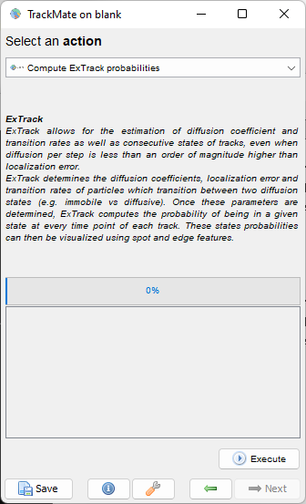
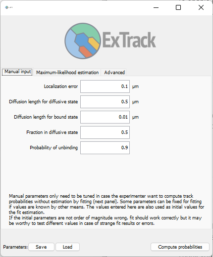
Select this action and click on the Execute button. The TrackMate-ExTrack UI window is shown:

Short tutorial.

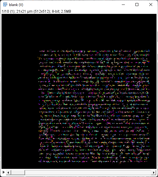
It is best explaining how ExTrack works with a short tutorial on synthetic data. Francois prepared 400 synthetic particles switching between diffusive and bound states and arranged them on a 20x20 grid. Then he saved the corresponding tracks as a TrackMate fle. You can get the TrackMate file (and more) on Zenodo:

We will work with the simulated_tracks.xml file first. This is a TrackMate XML file:

<?xml version="1.0" encoding="UTF-8"?>
<TrackMate version="7.7.2">
  <Log>Session log saved in the file
...</Log>
  <Model spatialunits="µm" timeunits="s">
    <FeatureDeclarations>
      <SpotFeatures>
        <Feature feature="QUALITY" name="Quality" shortname="Quality" dimension="QUALITY" isint="false" />

In Fiji,, go to the Plugins > Tracking > Load a TrackMate file menu item. Browse to the simulated_tracks.xml file. TrackMate will open the tracks, but because there is no image associated to it, you will see them in a blank image:

In the TrackMate window, click the Next button twie to move to the Actions panel. Select the action named Compute ExTrack probabilities and click the Execute button. The ExTrack window shown above should appear. The ExTrack interface is made of 3 panels: Manual input, Maximum-likelihood estimation and Advanced.

For ExTrack to work, it needs to estimate the values of several parameters:

• Localization error is a measure of the precision of spot location in physical unit.
• Diffusion length for diffusive state relates the diffusion coefficient of the first motility state, assumed to be the diffusive one. In 2D, it is equal to 2√Dt where D is the diffusion coefficient and t the frame interval.
• Likewise, Diffusion length for bound state relates to the second motility state, assumed to be the stuck one.
• Fraction in diffusive state is the average fraction of particles that are in the first state, the diffusive one.
• Probability of unbinding is the probability for a particle to go from the bound state to the diffusive state in the frame interval.

The first panel allows for manually entering the values of these parameters if they are known. Of course, the values are known only in ideal cases, and this is why ExTrack offers a means to estimate them solely based on the particles motion.

Move to the second panel, Maximum-likelihood estimation. Click the Start estimaton button. The process relies on maximum-likelihood estimation (MLE) and uses the values entered manuall as a starting guess. ExxTrack is relatively robust, so if the starting values are not too far off, the MLE should converge. The estimation can be long; with thes 400 tracks it takes about 1 minute on my 2021 workstation, but the starting values were close. We took advantage of multi-threading to speed up the iterations so you should hear the fan in your computer making noise.

Here are the estimates I obtained:

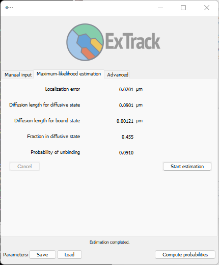
Your values should be close, but need not to be equal. We see that indeed, the bound state is found to have a smaller diffusion length than the other state. You can save the parameters to a JSon file using the Save button at the bottom left of the window. It will generate a simple text file that looks like this:

{
  "localizationError": 0.020066601029511685,
  "diffusionLength0": 0.09013966560752623,
  "diffusionLength1": 0.0012129577182051934,
  "F0": 0.45455903522933716,
  "probabilityOfUnbinding": 0.09100120643275995,
  "nbSubteps": 2,
  "nFrames": 5
}

You can later reload it with the Load button.

Now the hardest part is done. You can use these parameters to have ExTrack estimate what is the probability for a particle to be in a state or in another. Click the Compute probabilities button in the bottom right to do so. This computation should be relatively quick.

Once the computation is over, it pushes new numerical features to the TrackMate session. For instance, if you go back to the main TrackMate window, and click the Spots button in the Display options panel, you will see that the spots have now two new numerical features, P stuck and P diffusive:

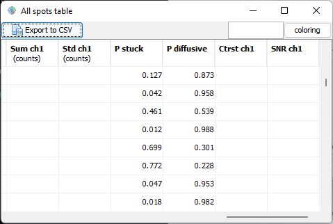
These numerical values can be used to generate a visualization of the current state in TrackMate. In the same TrackMate panel, in Color spots by, choose Probability diffusive under the Spot features category. Do the same for the Color tracks by settings. Click on the two auto buttons next to the min and max to have the display range automatically set from 0 to 1.

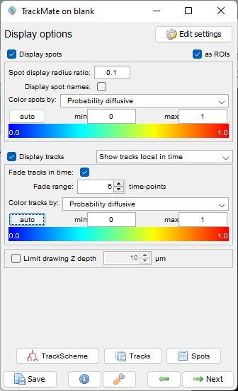
The colors should be reflected on the track display:

We can see particle transitionning from one state to another. On this simulated dataset, the probabilities of a state correspond well to the intuition give by the apparent displacement of the particles.

Note: The steate meanings can be inverted. Depending on the starting parameters and the estimation, it is possible that the state dubbed diffusive will actually represent the stuck one. We chose a convention where the state names are made explicit, but ultimately, whether the first state is diffusive or bound is determined by the value of the diffusion length.

Scripting TrackMate-ExTrack.

As most of the TrackMate ecosystem, ExTrack can be scripted using Jython. Here is an example script:

import os
import time

from java.io import File

from fiji.plugin.trackmate.io import TmXmlReader

from fr.pasteur.iah.extrack import ExTrack
from fr.pasteur.iah.extrack.compute import ExTrackParameters


def process( path ):

        # Load tracks.
        print( "Loading " + path )
        reader =  TmXmlReader(  File( path ) )
        model = reader.getModel()
        if not reader.isReadingOk():
                print( "Problem reading the file:" )
                print( reader.getErrorMessage() )
                print( "Aborting." )
                return

        print( "Loading done." )

        # Create an ExTrack object.
        extrack = ExTrack( model )

        # We only estimate parameters if we do not have them already saved.
        parent = File( path ).getParent()
        savefile = File( parent, "extrack-params.json" )
        if savefile.exists():
                print( "\nFound an existing save-file for parameters. Skipping parameter estimation." )

        else:
                # Estimate motility parameters.
                print( "\nEstimating motility parameters (can be long)..." )
                # Use the default as starting point.
                startpoint = ExTrackParameters.create() \
                                        .localizationError( 0.02 ) \
                                        .diffusionLength0( 0.001 ) \
                                        .diffusionLength1( 0.1 ) \
                                        .F0( 0.5 ) \
                                        .probabilityOfUnbinding( 0.1 ) \
                                        .nbSubSteps( 1 ) \
                                        .nFrames( 6 ) \
                                        .build()
                print( "Using the following as starting point:" )
                print( startpoint.toString() );

                start = time.time()
                optimum = extrack.estimateParameters( startpoint )
                end = time.time()
                print( "Estimation done in %.1f seconds.\nFound the following optimum:" % ( end - start ) )
                print( optimum.toString() )

                # Save.
                print( "\nSaving the parameters to a JSon file." );
                ExTrack.saveParameters( optimum, savefile.getAbsolutePath() )
                print( "Saved to " + savefile.getAbsolutePath() )

        # Load.
        print( "\nLoading the parameters from a JSon file." )
        loadedparams = ExTrack.loadParameters( savefile.getAbsolutePath() );
        print( "Loaded from " + savefile.getAbsolutePath() )
        print( "Parameters loaded:" )
        print( loadedparams )

        # Predict probabilities.
        print( "\nPredicting diffusive & stuck probabilities..." )
        extrack.computeProbabilities( loadedparams )
        print( "Done." )

        # Print probabilities.
        print( "\nContent of model features now:" )
        print( "-----------------------------------------------------------------" )
        print(  "| %-25s | %-15s | %-15s |" % ( "", "P stuck", "P diffusive" ) )
        print( "-----------------------------------------------------------------" )
        allspots = model.getSpots()
        frames = allspots.keySet()
        for frame in frames:
                print( "Frame " + str( frame ) + ":" )
                spots = allspots.iterable( frame, True )

                for spot in spots:
                        print( "| %-25s | %-15.3g | %-15.3g |" % ( spot.getName(), spot.getFeature( "EXTRACK_P_STUCK" ), spot.getFeature( "EXTRACK_P_DIFFUSIVE" ) ) )
                        break # Remove to get all spots.
                print( "-----------------------------------------------------------------" )
                break # Remove to get all frames.


if __name__ == "__main__":
        print( 'Current working dir: %s' % os.getcwd() )
        # Path to the TrackMate file containing your tracks.
        path = "scripts/samples/tracks.xml"
        process( path )

You need to modify the line 95 to have the path variable point to a TrackMate XML file. Here is the output of the script with the same simulated dataset we used in the tutorial above:

Started ExTrackScritExample.py at Wed Jul 20 10:53:09 CEST 2022
Current working dir: C:\Users\tinevez\Development\Fiji.app
Loading /Users/tinevez/Development/TrackMateWS/TrackMate-ExTrack/samples/simulated_tracks.xml
Started ExTrackScritExample.py at Wed Jul 20 10:54:40 CEST 2022
Current working dir: C:\Users\tinevez\Development\Fiji.app
Loading /Users/tinevez/Development/TrackMateWS/TrackMate-ExTrack/samples/simulated-tracks.xml
Loading done.

Estimating motility parameters (can be long)...
Using the following as starting point:
fr.pasteur.iah.extrack.compute.ExTrackParameters@132517e5
 - Localization error                   : 0.0200  
 - Diffusion length for diffusive state : 0.00100 
 - Diffusion length for bound state     : 0.100   
 - Fraction in diffusive state          : 0.500   
 - Probability of unbinding             : 0.100   
 - Number of sub-steps for optimization : 1
 - Number of frames for optimization    : 6

Estimation done in 27.8 seconds.
Found the following optimum:
fr.pasteur.iah.extrack.compute.ExTrackParameters@56c79383
 - Localization error                   : 0.0201  
 - Diffusion length for diffusive state : 0.00139 
 - Diffusion length for bound state     : 0.0908  
 - Fraction in diffusive state          : 0.555   
 - Probability of unbinding             : 0.0744  
 - Number of sub-steps for optimization : 1
 - Number of frames for optimization    : 6


Saving the parameters to a JSon file.
Saved to C:\Users\tinevez\Development\TrackMateWS\TrackMate-ExTrack\samples\extrack-params.json

Loading the parameters from a JSon file.
Loaded from C:\Users\tinevez\Development\TrackMateWS\TrackMate-ExTrack\samples\extrack-params.json
Parameters loaded:
fr.pasteur.iah.extrack.compute.ExTrackParameters@14de5359
 - Localization error                   : 0.0201  
 - Diffusion length for diffusive state : 0.00139 
 - Diffusion length for bound state     : 0.0908  
 - Fraction in diffusive state          : 0.555   
 - Probability of unbinding             : 0.0744  
 - Number of sub-steps for optimization : 1
 - Number of frames for optimization    : 6


Predicting diffusive & stuck probabilities...
Done.

Content of model features now:
-----------------------------------------------------------------
|                           | P stuck         | P diffusive     |
-----------------------------------------------------------------
Frame 0:
| ID0                       | 0.872           | 0.128           |
-----------------------------------------------------------------

JYT, July 2022