An ImageJ plugin for intensity-based three-filter set (ratiometric) FRET which works with unknown varying donor/accepter ratios, corrects for channel crosstalk and instrument calibration, and yields quantitative FRET E values.
Introduction
Assesment of molecular interactions is often based on Förster (fluorescence) resonance energy transfer (FRET). Several methods rely on measuring fluorescence intensities of the donor and acceptor to determine the extent of FRET from donor quenching and/or sensitized acceptor emission. Many of these arrive at FRET indices which are semiquantitative, qualitative, or outright ignorant of actual donor-acceptor ratios. The 3-cube approach is based on measuring donor emission upon donor-specific excitation, acceptor emission upon acceptor-specific excitation and acceptor emission upon exciting the donor. Properly describing the sources of the signal in each channel – taking spectral crosstalk, instrument sensitivity, and varying donor-acceptor ratio into account – allows for deriving a quantitatively correct expression for FRET efficiency. This approach has been implemented in the RiFRET plugin for analysis of microscopic images. The current version also incorporates pixel-by-pixel autofluorescence correction and batch mode analysis of large datasets.
Installation
- Download the latest version of Fiji.
- Enable the FRET Imaging update site.
- Once installed, go to Plugins > FRET Imaging > RiFRET.
Usage
Download the help file as a PDF here.
Table of Contents
Menu bar
File
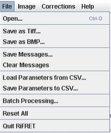
Open
Opens an image with the file manager.
Save as Tiff
Saves the selected image in tiff format.
Save as BMP
Saves the selected image in BMP format.
Save Messages
Saves the content of the messages pane in .txt format.
Clear Messages
Clears the messages pane.
Load Parameters from CSV
Loads previously saved calibration factors, thresholds, background values and radiuses for blurring to be used for either batch or manual evaluation.
Save Parameters to CSV
Saves for future use the calibration factors, thresholds, background values and radiuses for blurring that have been optimized for a given measurement/dataset.
Batch Processing
Opens the batch processing dialog (described later)
Reset All
Resets the appearance of the buttons for previously completed steps, and “clears” the previously “set” donor, transfer, acceptor, AF images – potentially useful if a user sets the channels incorrectly. It might also be useful after a batch processing run is complete. Parameters in the text fields are intentionally preserved – it is best to close and open the program again to clear these.
Image
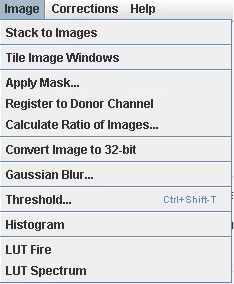
Stack to Images
Splits the selected multichannel image so each channel is treated as a standalone image. The resulting windows can be used during the analysis process by assigning to them the appropriate role at the steps using the “set image” function.
Tile Image Windows
Set the opened images to tiled view.
Apply Mask
Applies a selected 32-bit image created from a 32-bit image by thresholding (which contains NaN pixels) as a mask to another image. Any grey values different from NaN are taken as unity in the mask image. The image to be masked is automatically converted to 32-bit when the “Set image to be masked” command is applied. The two images must be the same size. The command opens this dialog:
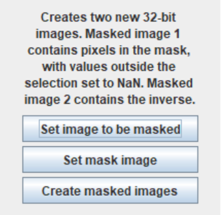
Setting the input images renames them as “Mask image – date” and “Image to mask – date”. The output images are 32-bit and named:
Masked image 1 (pixels in the mask)
Masked image 2 (pixels outside the mask)
Register to Donor Channel
This will register the transfer and acceptor channels to the donor channels in 2D (registration of the autofluorescence channel is not supported owed to the expected lack of its correlation with labels). Image registration is performed using an implementation of the Fast Hartley Transform (FHT). Images are first duplicated, forward transformed into the frequency domain, conjugate multiplication is then performed (this is equivalent to cross-correlation in the spatial domain). Finally, images are inverse transformed back into the spatial domain. The maxima (peaks) are then used to shift in X and Y. Currently, sub-pixel shift is not supported. N.B. Image registration requires image dimensions to be 2n and square (e.g. 512×512). Results of registration will be output to the log.
Calculate Ratio of Images: Calculates the ratio of two selected 32-bit image
Convert Image to 32-bit: converts images to 32-bit format.
Gaussian Blur
Applies a Gaussian blur with a selected σ 1/e2 radius. (Former users of RiFRET please note that the Gaussian Blur used in versions 1.x had 2.5 times larger radiuses with the same value set, and it is now deprecated.)
Threshold
Opens the FIJI built in threshold function. N.B. Needs 32-bit images to set over and/or under values to NaN
Histogram
creates a histogram of the selected image
LUT fire
Applies the fire lookup table to the selected image
LUT spectrum
Applies the spectrum lookup table to the selected image
Corrections
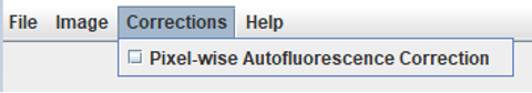
Pixel-wise Autofluorescence Correction: Enables the pixelwise autofluorescence function. (Changes the main window of the plugin)
Using the Plugin with pixel-wise autofluorescence correction
Main window with pixel-wise autofluorescence correction
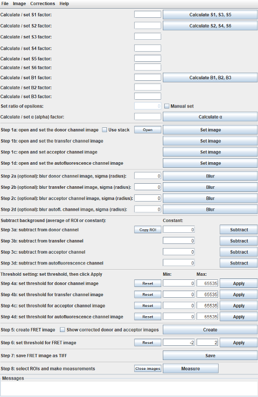
Calculate correction and calibration factors
These factors can be entered manually or calculated from images using the calculate buttons.
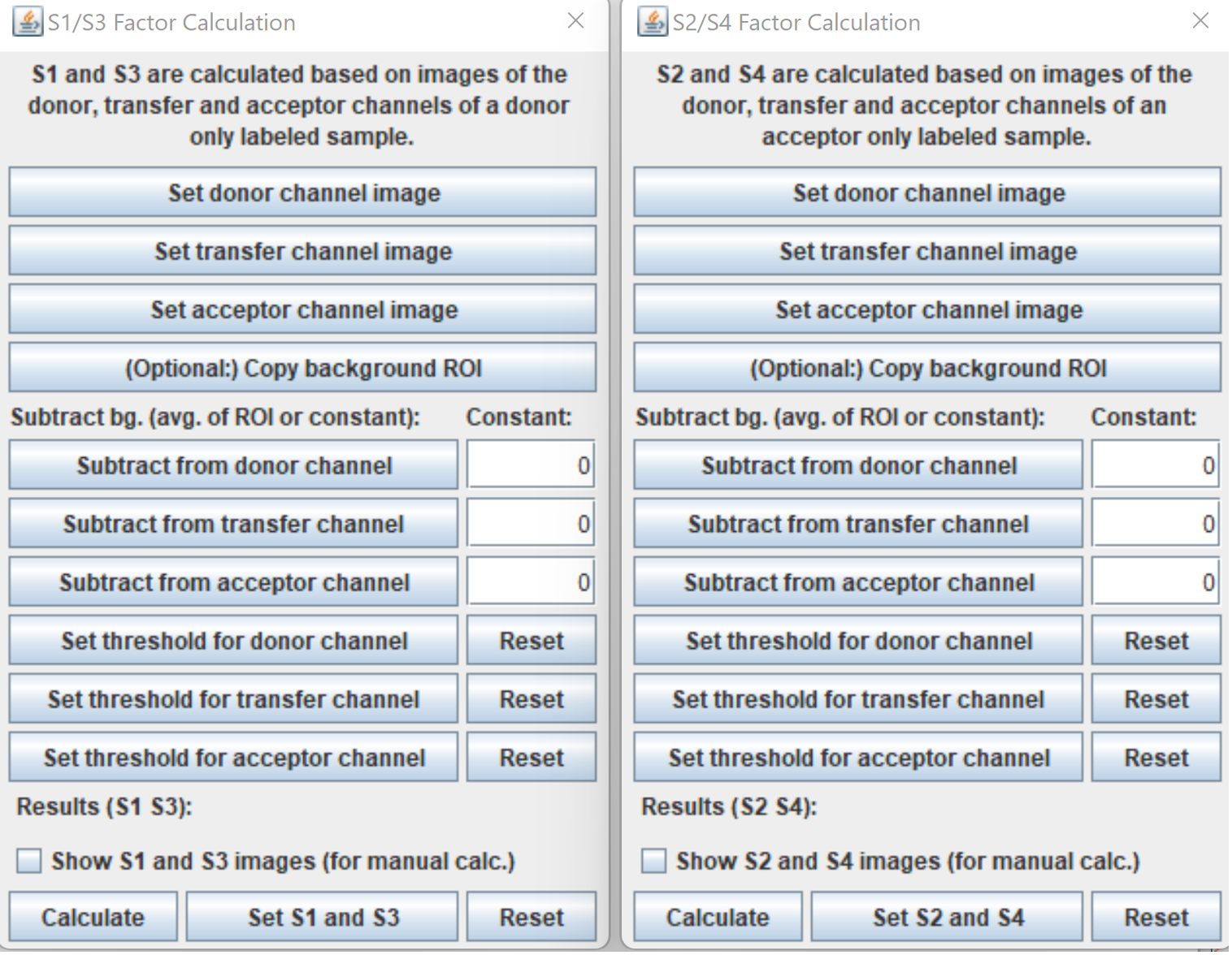
Calculate S and B factors
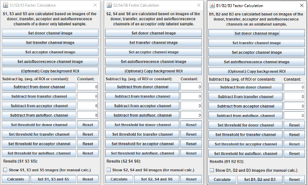
All windows implementing the calculation of spectral spillover factors (S and B factors) follow the same logic. The S1, S3, S5 factors can be calculated on a donor only sample, the S2, S4, S6 factors on an acceptor only sample and the B1, B2, B3 on a non labelled sample.
First, the fluorescent channels should be set. If only stacks are available, use Stack to Images. When the single-channel images are available select the donor channel then click on the Set donor channel image button. Repeat this step with the other channels. All images are set to 32-bit depth automatically.
Background subtraction
Donor only and acceptor only samples can be both cell-free standards or labeled cells (see manuscript). Samples for B factors should be the same cells that FRET will be measured on, but without labelling.
For each channel, there are two options for defining the value to be subtracted.
Option 1: select a ROI with the FIJI built in options in the donor channel in the case of S1, S3, S5 in the acceptor channel in the case of S2, S4, S6, and in the autofluorescence channel in the case of the B factor window. Click on the button (optional:) Copy background ROI. The selected ROI will be copied to all the channels.
Option 2: If the background value is known you can type it into the boxes under the text Constant:
When clicking on subtract for each channel, the plugin checks if there is a ROI in the image and subtracts the average value of the ROI and also subtracts the constant. So depending on the samples used for the S and B factors, either the ROI average or the constant should be used.
(i) For obtaining the S factors from cell-based samples, the background ROI should be on a cell-free part of the image and only the instrument background (including constant noise, reflections from surfaces, etc.) will be subtracted. This only works if the autofluorescence of the sample is negligible compared to signal, which may be achieved by using cells with low AF and high expression levels for the S factors, even if FRET will be measured on low expressing and/or high AF cells. In this case, the constant should be kept 0.
If S factors can only be determined on labeled low expressing and/or high AF cells, average background of the same cells, but without labeling, needs to be determined and entered as constant. In this case, no active ROI should be present. (For this approach, the sample used for the B factors can be used).
(ii) The optimal solution is to use cell-free calibration samples for the S factors (see manuscript). In this case, instrument background should be determined on an equivalent slide with no fluorophores, and entered as a constant, while at the same time no ROI should be active.
(iii) For B factors, the same sample that FRET will be measured on - but without labeling - needs to be used. Here, the background ROI should be on a cell-free area and the constant should be 0, or no ROI should be active, and an independently measured instrument background entered as constant. Make sure background ROIs contain no cells when using pixel-wise AF correction.
The threshold buttons open the built in Threshold window of Fiji. After selecting the appropriate threshold, it should be applied and the Set to NaN option should be selected. The selected threshold can be reset with the reset.
When the show images (for manual calc.) box is checked, the plugin displays the result images, otherwise it provides the results only.
With Calculate the results can be generated.
The set (S1, S3, S5, etc.) apply the calculated values in the main window.
The reset resets the steps in the window for a new calculation.
Set the ratio of epsilons
The value is normally ~0. For calculating an exact value for the dye
pair and lasers used, see (Manuscript, Eq. 5)
\(epsR = \frac{\varepsilon_{A.exc}^{D} \bullet \varepsilon_{D.exc}^{A}}{\varepsilon_{D.exc}^{D} \bullet \varepsilon_{A.exc}^{A}}\)
The epsR is the product of the ratios of the donor and acceptor dye’s
molar absorption coefficients at each other’s excitation wavelengths to
their absorption coefficients at their own excitation wavelengths. For
most dye pairs this numeric is negligibly small.
Calculate α
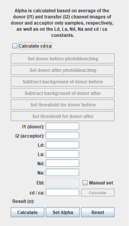
For calculating the alpha factor, the intensity of the donor channel (I1) on a donor only and transfer channel (I2) on an acceptor only sample are needed. You can use the same images for I1 and I2 as for the S1/S3/S5 and the S2/4/6 factors, respectively. After selecting the appropriate window, press the “M” key to measure and copy/paste the result to the dialog.
Ld is the mean number of dyes attached to the donor antibody
La is the mean number of dyes attached to the acceptor antibody
Nd: the mean number of receptors labelled by the donor on the cells
Na: the mean number of receptors labelled by the donor on the cells
εd/εa: Is the ratio of the molar absorption coefficient of the donor dye / the acceptor dye at the wavelength of the donor excitation. These can be calculated using the spectral data of dyes and instrument light sources.
When these data are not available, they can be calculated based on an acceptor photobleaching experiment and activating the option „Calculate εd/εa”. The donor before and after photobleaching should be set, the background and threshold values adjusted and then the “calculate” button next to the εd/εa text box.
Since calculating the actual FRET E from an acceptor photobleaching experiment usually necessitates various corrections, a fully corrected Ebl value can be obtained by using on the same set of input data the AccPbFRET plugin (see REFs). In this case, the Manual set at the Ebl input dialog should be selected.
Please note that determining the alpha factor in this manner is only a reasonable approach when the autofluorescence of labeled cells is negligible compared to the fluorescence signal. For best results, the use of standard slides with labeled proteins but no cells, and the use of exact spectral data for εd/εa are recommended.
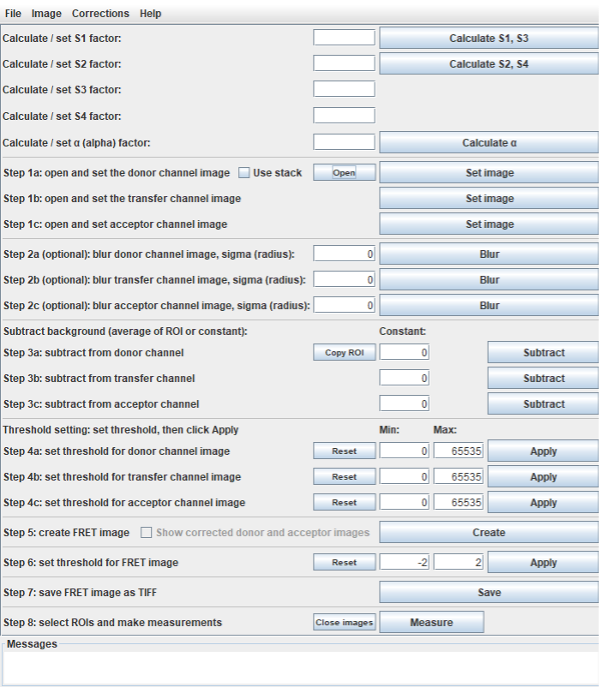
Calculating FRET
When all the correction factors are determined, FRET E can be calculated on double labeled samples.
Step 1: Open and set images
The double labeled images should be opened.
Open and set as channels:
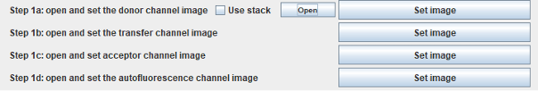
with open the built-in image opener of Fiji starts (all the supported image formats can be opened this way). If images are in stacks, they can be split using Stack to Images in the IJ menu.
When single channel images are opened, select the window with the donor channel and click on Set image at step 1a. Continue with the transfer, acceptor, and autofluorescence channels in the same manner.
Step 1: Open stacks
When the Use stack is checked, the main window changes:
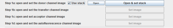
Click Open & set stack, The built-in image opener of Fiji starts. Select a stack, and when it is opened, the following window should appear:
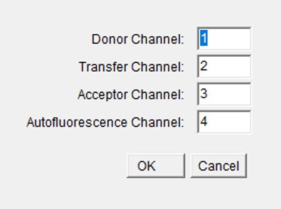
The position of the appropriate channel in the stacks should be written
in the dialogue boxes in a numeric form. The numbering of channels
starts with 1.
Click on OK and the image stack is split and the resulting windows are
properly named.
Step 2: Blur channels
Optional step, with the dialogue box, the pixel radius of the blurring can be entered. The plugin uses the Gaussian Blur function of the FIJI. It can be a useful tool when only low SNR images are available. (Please note that all the channels should be blurred with the same radius)
Step 3: Subtract background
The background subtracted here should only be the instrument background including constant noise, reflections from surfaces, etc. Autofluorescence from cells or tissues is taken into account on a pixel by pixel basis using the B factors calculated previously.
Option 1: select a cell-free ROI with the FIJI built in options on the donor channel, and click on Copy ROI. The selected ROI will be copied to all the channels.
Option 2: If the background values are known from an independent cell-free sample, you can type them to the boxes under the text Constant:
Please note: When clicking on subtract for each channel, the plugin checks if there is an active ROI in the image and subtracts the average value of the ROI and also the constant. So if a background ROI is selected, the constants should be kept 0, and if the non-zero constants are used, please do not select a background ROI.
Step 4: Thresholding
Setting threshold for the measured fluorescence channels. The min and max values can be defined for all the fluorescence channels. With the apply button, the pixels outside the given maximum and minimum range will be set to NaN. FRET E values are only calculated on numeric values, so if pixel is NaN in any of channels, it is set to NaN in the FRET E image as well. With the Reset button, all pixels are reset to their original value of before any threshold operation.
Step 5: Create FRET Image
FRET E images can be created with the Create button. When the Show corrected donor and acceptor images box is checked, also FRET E and spectral spillover and autofluorescence corrected donor and acceptor images are created.
Step 6: Set threshold for FRET image
The min and max values can be defined for the FRET E channel. With the apply button, the pixels outside the given maximum and minimum range will be set to NaN. With the Reset button, the non thresholded FRET E image can be reloaded.
Step 7: Save FRET image as TIFF
Saves TIFF format images with the built in FIJI image exporter
This command also saves the corrected donor and acceptor images into a stack when the show corrected donor and acceptor images option is activated.
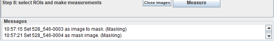
Step 8: Select ROIs and make measurements
With the measure the whole FRET E image or the active ROI marked within is measured. RiFRET creates a custom results table with a custom implementation for calculating the Number of Pixels, Not NaN Pixels, Mean, Median, SD, Min and Max. Please note that the list of calculated parameters is fixed, IJ/FIJI preferences for its built in “measure” function do not affect the results. These result also may have different levels of precision to those calculated by IJ/FIJI.
To measure multiple ROIs, the FIJI built-in ROI manager and measure functions need to be used.
The close image button closes both the original and the calculated images.
Using the Plugin without pixel-wise autofluorescence correction
Main window without pixel-wise autofluorescence correction
Without pixel-wise autofluorescence correction, the main window does not display the boxes for B factors, and the button to set the autofluorescence channel. Other differences from pixel-wise AF correction are highlighted below.
Average autofluorescence correction
This mode of the plugin offers an alternative autofluorescence correction method wherein the average autofluorescence is used. These values for each channel, comprised of both cellular/tissue AF and instrument background, can be entered as a constant after determining them using unlabeled cellular /tissue samples with the same exposure settings. (Same samples as one would use for determining the B factors for pixel-wise correction.) We only recommend the average correction method with cellular data if cellular autofluorescence is spatially homogeneous.
Alternatively, cell-free ROIs can be used in the FRET images, however this will only correct for instrument background including constant noise, reflections from surfaces, etc.. This is only recommended for the cases where cellular/tissue autofluorescence is negligible compared to label signals.
Calculate S factors
Of the S factors, without pixel-wise autofluorescence only factors S1-4 need to be determined.
Background subtraction
See above, except only S1/S3 and S2/S4 are calculated and only images for these are opened and used.
Batch processing
The batch processing works with every image format compatible with FIJI. When starting work on a new dataset, it is recommended to first do an analysis going through the entire procedure manually and verify that all parameters are correct.
The parameters of the analysis can then be saved to a CSV file: File > Save Parameters to CSV.
The parameters of the analysis can be loaded from a CSV file File > Load Parameters from CSV.
When a CSV is loaded or the parameters are otherwise determined in the main window, the batch processing can be started. File > Batch Processing
1. When the window describing the batch processing appears click OK (should read the contents first)
2. Select the input directory.
3. Select a CSV with the appropriate parameters. To keep and use the parameters currently displayed in the main window, simply click cancel.
4. Set the channel order numerically and click OK (see above)
The plugin will produce and measure the FRET images with the selected threshold values. The FRET images and the corrected channel images (if this option is selected) will be saved to a directory named Output within the parent input directory (this will be created if it does not exist).
Citation
This software is based on a publication. If you use it in your work, please cite:
See also
If you are using the acceptor photobleaching FRET method, we recommend our other FRET plugin AccPbFRET.