The FLIMJ plugin for ImageJ provides the ability to analyze FLIM data within ImageJ, using the FLIMLib library. The plugin can be installed into the Fiji distribution of ImageJ simply by enabling the FLIMJ update site. Features include:
- Fit individual pixels, entire images per-pixel, or do global analysis on entire images, using FLIMLib’s rapid lifetime determination (RLD), Levenberg-Marquardt (LMA) or global analysis (Global) fitting algorithms
- Single, double and triple exponential fits
- Gaussian, Poisson and Maximum Likelihood Estimation noise models
- Produce one or several fitted images depending which parameters (A, τ, Z, χ²) are chosen for visualization
- Full control over the start and end fit cutoffs known as “cursors”
- Binning options for various kernel sizes to reduce noise and boost intensity when fitting per-pixel
- Support for so-called “excitation” or “prompt” files containing a recorded system response function to be convolved with the exponential fit
- Batch processing support for analyzing many lifetime images as part of a scripting workflow
Installation
The FLIMJ plugin is available from the “FLIMJ” update site.
Once you have installed the FLIMJ plugin, it becomes available on the menu under Analyze › Lifetime › FLIMJ.
Usage
Startup
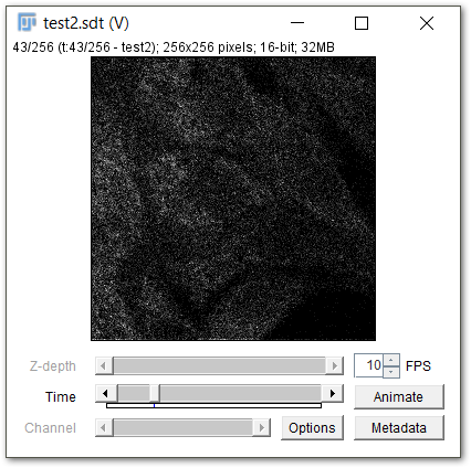
Open a dataset (such as this one) or select an existing image display in Fiji:
With the desired dataset window active, launch FLIMJ from the menu under Analyze › Lifetime › FLIMJ or search for “FLIMJ” in the search box:
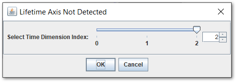
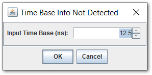
FLIMJ plugin accepts only 3- or 4-dimensional datasets. If the dataset is opened from a file supported by SCIFIO (such as a .sdt), the dataset likely has metadata attached, which helps FLIM plugin infer the order of the X, Y, and T axes as well as the time bin size. Otherwise, the user may be asked to provide the information:
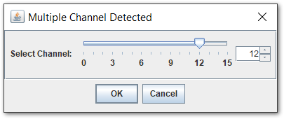
If the dataset comes with a (fourth) spectral dimension, the user has to choose the spectral channel to analyze as well:
Fit preview
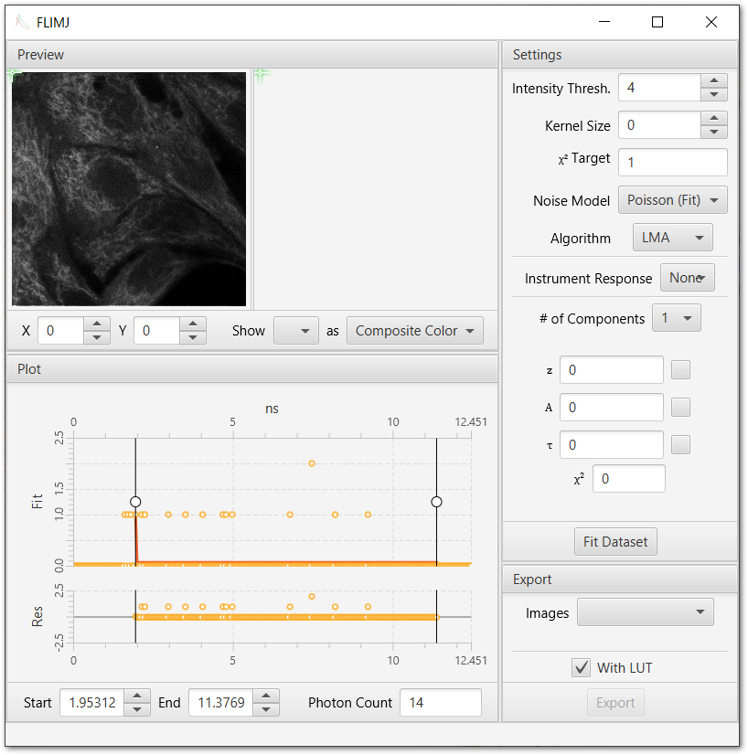
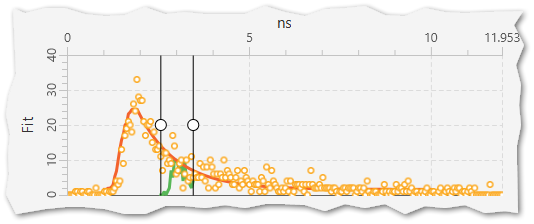
Before fitting the entire dataset, the user may click on the intensity image or type in the coordinates in Preview panel to preview the fitted curve and parameters of the pixel under the cursor:
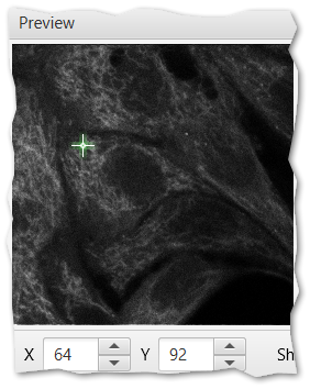
In the screenshots above,
- X and Y are coordinates of the pixel cursor counting from the upper left corner.
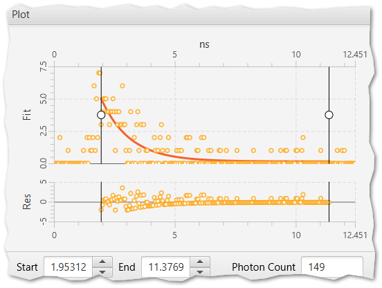
- Red curve denotes the fitted portion of decay between the start and end cursor.
- Orange dots denote the photon counts in each time bin in Fit plot and denote the residual (\(y_{data}-y_{fit}\)) in Res plot.
- Photon Count displays the total number of photons collected between the start and end cursor.
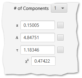
- \(z, A, \tau\) (or \(z_1, A_1, A_2, \tau_1, \tau_2\) in two-component fit) are the background, initial intensity and lifetime parameters of the model.
- \(\chi^2\) shows the chi-squared measure of the fit (see Noise models).
Fit settings
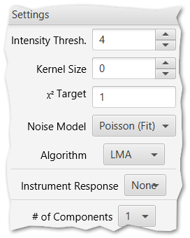
Options on the Settings panel.
Sometimes you may want to fine-tune the fitting configurations. The Settings panel and the Plot panel. The configurations include:
-
Intensity Thresh.: The minimal pixel intensity to be fitted.
Any pixel with cumulative intensity (over all time bins) below this threshold will be skipped when the dataset is fitted. When selected for preview in the Preview panel, only the photon counts (orange dots) will be plotted. For those pixels, all parameters are treated as 0 both when being previewed and when the whole dataset is fitted. -
Kernel Size: The radius (in pixels, excluding the center) of the binning kernel.
FLIMJ plugin currently only supports the square kernel with size \(2r+1\) and values all equal to 1 where \(r\) is the radius). The binning of the dataset is performed by convolving the dataset with this kernel, which is equivalent to adding neighboring pixels into the center:
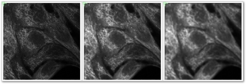
Left to right: Intensity of dataset after binning of radius 0, 1, and 2.
-
χ² Target: The \(\chi^2\) value below which the LM fitting will stop.
The LM algorithm checks at the end of each iteration whether the fit is good enough by comparing \(\chi^2\) with this threshold. If the results are satisfactory, the LM algorithm will terminate. -
Noise Model: The noise model used for fitting (see Noise models).
- Algorithm: The algorithm used for fitting.
Currently supported algorithms are:- LMA: The Levenberg-Marquardt algorithm;
- Global: The global LMA algorithm;
- Bayes: The Bayesian fitting algorithm.
-
Instrument Response: The dataset that contains the instrument response. (see Instrument response function (IRF/prompt))).
-
# of Components: The number of exponential decay terms in the model.
FLIMJ plugin currently supports up to 3 components. - Start and End: The ends (in ns, inclusive) of the interval during which the data is considered.
The cursors can be changed by dragging in the Fit plot, clicking on the up and down buttons, or typing in values (input will be rounded to the nearest time bin marking).
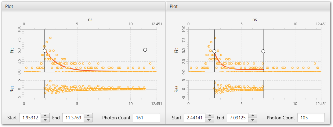
Change of the cursors results in different fit results.
Instrument response function (IRF/prompt)
FLIMJ plugin currently only supports the selection of IRF from a single pixel in an acceptable dataset that is taken during a standard IRF measurement procedure (such as this one using urea crystals). The steps are as follows:
-
Click on the drop-down menu, select From file; select the dataset file that contains the IRF.
-
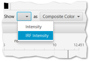
In Preview panel, select IRF Intensity for the “Show” option (you may also select Grayscale for the “as” option to deactivate pseudocoloring):
-
Click on the image to select the candidate pixel and drag the Start and End cursors in Plot panel to crop out the section of interest (IRF is plotted in green):
-
Exit the IRF picking mode by selecting other options for the “Show” in Preview panel and adjust the Start cursor to get a better fit.
You may readjust the IRF by starting from step 2 above. You may also reset the IRF setting by selecting None for Instrument Response in Settings panel or go back to a previously set IRF by choosing the corresponding filename there.
Dataset fitting and results preview
When all settings are properly configured. Click on button on the Settings panel to start dataset fitting. A “pending” progress indicator will appear on top of the button.
After the “pending” state ends, new options will be available as “Show” options in the Preview panel. Click on the options to view the fit results:
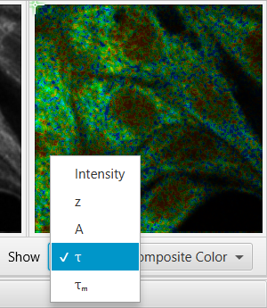
Viewing the \(\tau\) (lifetime) parameter of the fitted dataset.
You may also change the “as” option to specify how the results are rendered. Currently supported options are:
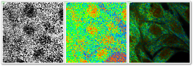
Left to right: The \(\tau\) image rendered with Grayscale, Color and Composite Color.
-
Grayscale: Linearly maps the middle 80 percentile of the result image’s values to grayscale colors from black to white. Values below the 10th percentile and above the 90th percentile are rendered black and white respectively.
-
Color: Linearly maps the middle 80 percentile of the result image’s values to colors from
hsl(20, 100%, 50%)tohsl(220, 100%, 50%)(see color bar below). Out-of-range values follow the same rule as in Grayscale. -
Composite Color: Takes the color mapped to by Color but replace the brightness with the brightness of the intensity image (on the left of the Preview pane). This option makes the fitted image look more uniform by deemphasizing jittery low photon count pixels.
You can hover the mouse pointer on the rendered image to see the lookup table (LUT) color bar and the numerical value of the pixel:
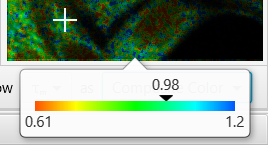
Hover on image to see the color bar, the pixel value, and its place in the range.
Image export
After dataset fitting, you can select images to export in the drop-down checklist on the Export panel.
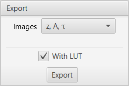
Options on the Export panel.
Hit button to export the selected images to for further processing. If “With LUT” is checked, the exported image will be loaded with the LUT used to render the preview image on the Preview panel (value ranges are set for each image separately).
You may follow the following steps to reproduce the composite color image after export:
- Export “Intensity” with desired fitted images;
- Convert all images to RGB format by searching and executing the “RGB Color” command in Fiji;
- Search and execute the “compose rgb-stacks” script, make the intensity image the “source” and the fitted image the “target”, and choose “Multiply” as “compose method”. Hit “OK”.
Advanced topics
Noise models
Documentation unfinished. For now, see the source code at:
And:
Publication
If you use FLIMJ in your work, please cite the paper: