SNT: Step-By-Step Instructions
| Home | Manual | Walk-throughs | Screencasts | Shortcuts | Rec. Viewer | Analysis | Scripting | Modeling | FAQ |
Contents
Tracing
These instructions assume that you have read the Overview page, including starting up the plugin, enabling Cursor Auto-snapping, and Auto-tracing options. This section is also documented in a Screencast.
Starting A Path
I. Pick The Starting Point
You may notice that, by default, the cursor snaps to the brightest pixel in its vicinity. If you prefer to manually control the placement of nodes, feel free to toggle feature by pressing S. Now, to begin tracing, move through the image stack to find the start point of a path then click there with the left mouse button.
II. Pick A Subsequent Point
A small circle should appear, highlighting the start of the path. Move through the stack to find a subsequent point further along the same structure to be traced (neuron, blood vessel, etc.), and click there.
If a path between the two points cannot be found immediately, you may see the animated progress of the search. You can scroll through the stack while such a search progresses: If it appears to not be making good progress, it's probably best to press the "Cancel/Esc" button (shortcut: C/⎋ Esc) and pick a point closer to the start point.
III. Confirm The Temporary Segment
Once the search has reached the target point, the path is shown in cyan (to indicate that this is still a temporary path) and you are asked to confirm (by clicking "Yes" or pressing Y) that this path is following the route through the image that you expect. If it is not, then click "No" N and you'll go back to the previous step. Assuming you confirmed the path, the confirmed path will appear in red. Now you are essentially back at step II. Normally you will go on to pick further points along the structure. However, if you have finished with that path, click "Finish Path" F and you will go back to step I. If you completed that path it would be shown in magenta.
Branching: Start A Path On An Existing Path
I. Select The Path To Branch Off
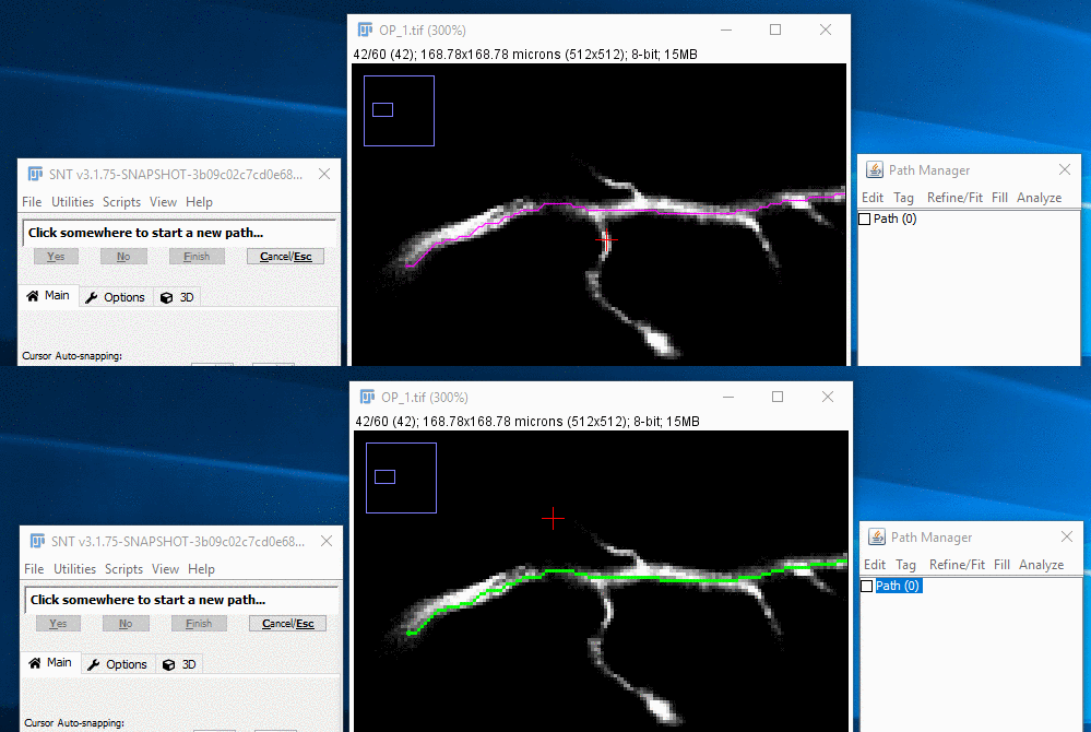
To select the path you want to branch off from, you can either select it in the Path Manager, or press G while the mouse pointer is near the path. When the path is first selected, it will be shown in the default green color.
II. Select The Fork Point
To force the start of the new path to be a branch of the selected path, hold down the ⎇ Alt+⇧ Shift keys while you move the mouse to find the branch point under the red cross-hairs, now decorated with a "Fork Point" annotation. With ⎇ Alt+⇧ Shift held down, click with the left mouse button. Finally, release the keys. Note that it is also possible to zoom into the branch point, right-click on the image and choose Fork at Nearest Node from the contextual menu.
III. Extend The Path
From this point on, you can carry on adding nodes to the branched path as above, i.e., Create a temporary path and confirm it. When you decide to complete the path you should see in the Path Manager that it has been recorded as a child of the existing path.
Joining: End A Path On An Existing Path
|
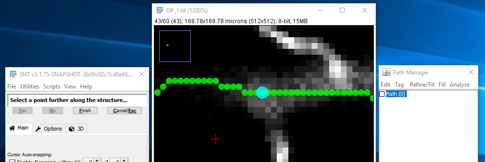
Supposing you want the end of a path that you're tracing to join onto an existing path, you just use the same modifier key when selecting the end point of the last part of the path. To go into that in more detail, if you're halfway through tracing a path like [1]: |
|
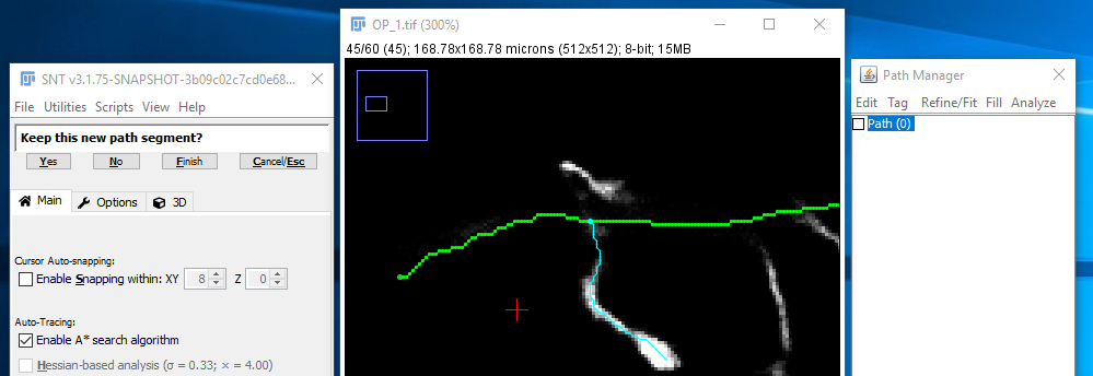
| ... and you want the final part of that path to join up with the existing path running from the top-left to top-right of the image. First, select that path in the path list (or using the G shortcut) as in [2]: | |
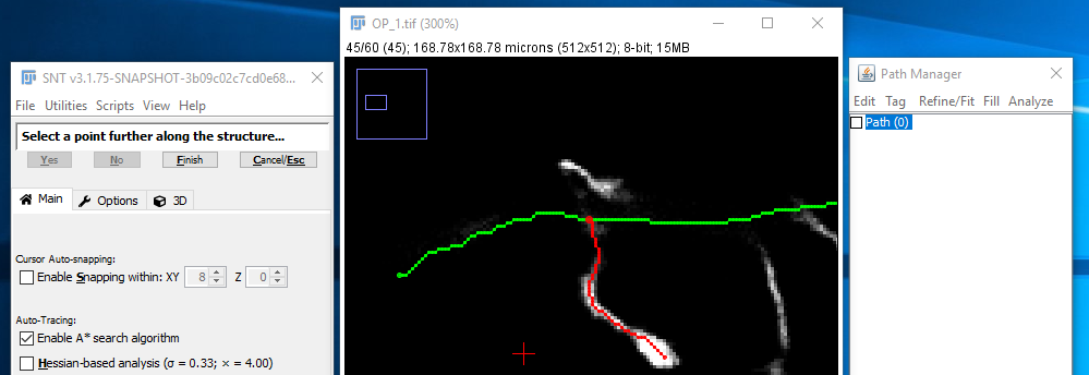
| Now hold down ⎇ Alt+⇧ Shift to restrict the endpoint to be a "join" on that existing path. Click (while still holding down the modifier keys) to start the search for that endpoint and make it join the existing path. If the search can find a path to the end point, the result should look like [3]: | |
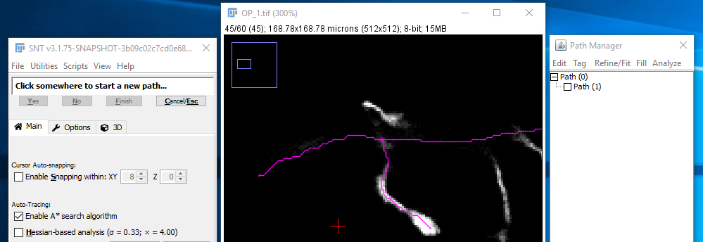
| If you're happy with the result, confirming the temporary path will automatically complete the whole path, since if you're creating an end join there cannot be any more to the path. Note that the path list indicates that this new Path (1) ends on the existing Path (0). The result will look like [4]: |
Merging/Joining Paths
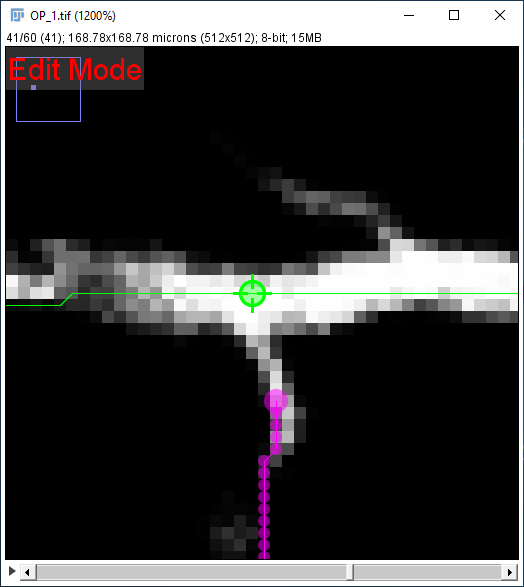
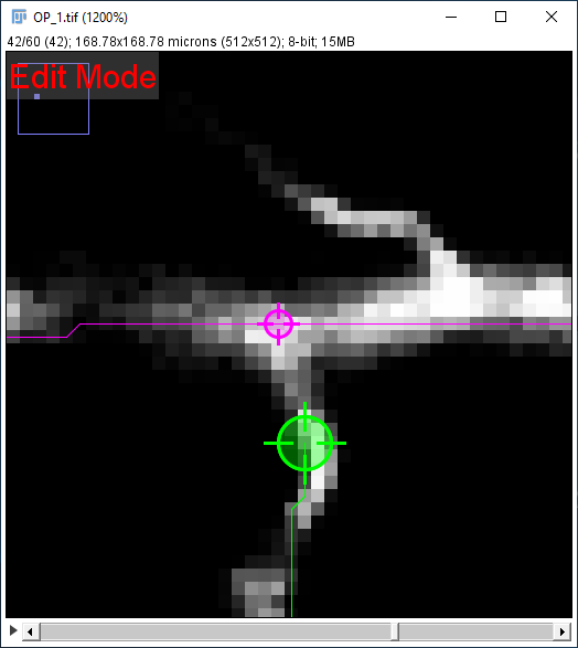
Two paths can be merged or joined in Edit Mode. To do so:
- Select a path and enter Edit Mode (by right-clicking on the image canvas to access its Contextual menu)
- Activate the node to be merged by hovering over it
- Select the second path by using the G shortcut and activate the second merging node by hovering over it
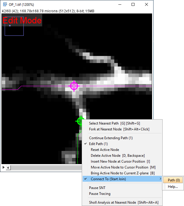
- Open the contextual menu and select the initial path from the Connect To (Start Join) / Connect To (End Join) menu.
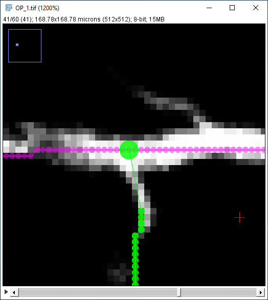
If both nodes are terminal, the paths are merged together. Otherwise, one path will become a child of the other. Note that one of the nodes must be terminal, to ensure no loops are created.
Tracing in the Legacy 3D Viewer
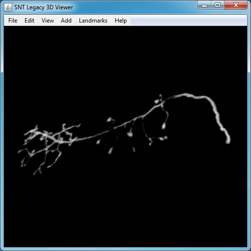
It remains possible to trace in the legacy 3D Viewer.
I.Starting the Viewer
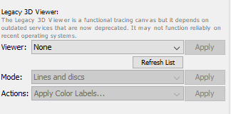
To open the viewer, select the 3D menu tab in the SNT dialog and look for Legacy 3D Viewer. You will see 3 parameters:
- Select New with image from the Viewer drop-down menu (selecting New without image would only allow you to look at reconstructions without the underlying signal). Note that you can recycle existing viewers you may have open by choosing their window titles from the drop-down menu.
- Select the preferred rendering style from the Mode drop-down menu.
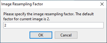
- Once you Apply the viewer choice, a prompt will appear asking you to choose the resampling factor for the image. Then, the viewer window will appear with the currently open image.
- Selecting points for tracing Select the Wand tool (W shortcut) in the main ImageJ toolbar and click over the region you want to trace. Tracing works the same way as in the 2.5D view, i.e., click somewhere in the image to create a starting point, then click further along the structure of interest to find a path between the two points, then confirm or deny the temporary segment as described above. Similarly, branching occurs as described for 2D canvas(es), by holding the ⎇ Alt+⇧ Shift modifier.
- Rotation Either use the Hand tool (H shortcut) tool and left-click while dragging the mouse or drag mouse while holding the scroll wheel.
- Translation Hold ⇧ Shift and the scroll wheel while dragging the mouse.
- Adjusting zoom depth Scroll the mouse wheel.
Once you have selected each of these tools (Wand and Hand) once, you should be able to switch between them by pressing the ⎋ Esc key. See Key Shortcuts for the list of all supported shortcuts.
Filling
There is a simple facility in this plugin for "filling out" paths to volumes. This is not particularly sophisticated, but often good enough for a rough visualization of the shape of a neuron beyond what can be seen from the traced path.
I.Starting the Fill
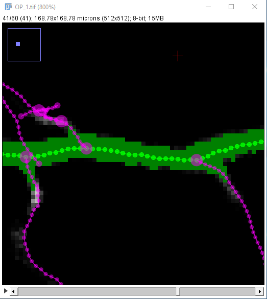
First, select the one or more paths that you want to fill out from in the Path Manager and select "Fill -> Fill Out..." in the Path Manager menu options. The selected paths are shown in green so that you can check that you're starting from the right ones. After a couple of seconds if you scroll through the stack you should be able to see a thick green surround the path:
The filler continues to explore the image starting from the path until you click "Pause" or "Stop" in the dialog. However, the fill which is shown only includes those points up to a certain threshold distance from the path. (Note that in this section "distance" doesn't mean a real physical distance, but a measure which takes into account the intensity values of the pixels which must be passed through when moving away from the path.) Information about the current threshold and the progress of the search is shown in the dialog.
The "Cursor position:" state under "Search Status" is updated as you move your mouse over the image. If the point under the mouse has been reached by the search then it will show you that point's distance from the path. Otherwise, it will read "Not reached by search yet". Two lines above, the "Current threshold distance:" shows your current threshold distance: so if this is set to 0.2 then that means that all points less than 0.2 from the path are included in the fill (and shown in green in the image.) The "Max. explored distance:" state under this line shows the maximum distance from the path that has been completely explored.
II.Adjusting the Fill Threshold
You can change the fill threshold in one of three ways:
- Clicking on a point in the image that has been reached by the search (This is the most intuitive way of altering the threshold). It may be helpful to disable the "Enable Snapping within: XY-Z" feature for the cursor while doing this.
- Manually changing the threshold in the "Specify manually:" input box and clicking the "Apply" button beside it.
- Clicking the "Use explored maximum" button below the threshold input box and click "Apply", which sets the threshold to the maximum explored distance (the value shown in "Max. explored distance:" under the "Search Status" dialog).
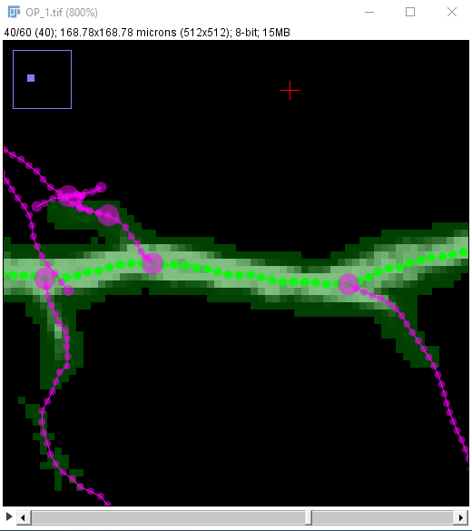
Anyway, assuming that you want to use the first of these approaches, you should use the approach described below. It is difficult to set the threshold accurately from the image unless you zoom in, so first zoom on part of the path that you want to set the threshold for.
Since the solid green fill obscures the intensity value of the points in the fill, I suggest that you switch to the semi-transparent view of the fill at this stage by selecting the "Transparent overlay" option in the "Rendering Options" dialog. Note that this may slow down filling.
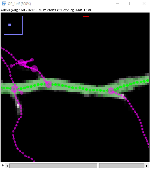
As you can see in the middle image, the threshold is set too far from the path, since there are many completely dark points under the green fill, as well as points on different paths than those of interest. Experiment with clicking on different points closer to the path in order to adjust the threshold until you are happy with it. You might end up with something like the rightmost image:
III.Completing the Fill
If you are happy with this, then you might as well click "Pause" so that your computer isn't spending all its CPU on continuing to explore the image. Then you can either:
- Save the fill (which will add it to the fill list) by clicking "Stash Progress".
- Discard the fill by either clicking "Stop" while filling is in progress or, if you stashed the fill, select it in the fill list and click "Delete Fill(s)".
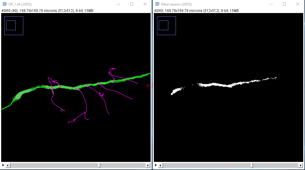
- Use the "Image Stack..." button to view the same image stack, but with only the points in that fill preserved. You can choose either a grayscale image or a binary mask. One reason why you might want to do this is that you can then smooth that image and use the 3D Viewer to do a surface rendering of the neuron. Perhaps then you could overlay that onto a volume rendering of the complete image (see available tutorials). Or, you could save those fill stacks for each of the neurons you fill and then combine them in ImageJ using "RGB Merge".
The image stack you would get from the image used in this example might look something like this:
Generating Filtered Images
This section describes how to generate Filtered Images outside SNT. Note that the filtering used in this walk-through (Frangi Vesselness) is already supported directly by SNT. This tutorial will assume you need to perform the filtering with adjusted parameters.
A Single Image
To process a single image with the Frangi Vesselness filter, pause SNT, and select Process › Filters › Frangi Vesselness. By way of example, let's say you need to enhance strucutres at two scales: twice the x voxel separation and five times that value. We apply a Gaussian convolution at each scale. Assuming your image has isotropic resolution with pixel width = pixel height = voxel depth = 1, the parameters would be:
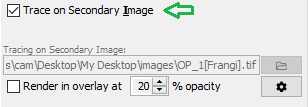
Save the result using File › Save As › Tiff... ("test-filtered.tif", for example). Then, in SNT's dialog look for the "Tracing on Secondary Image" widget in the Main tab. Click the file folder button to specify the secondary image. Next, toggle the "Trace on Secondary Image" checkbox (you can do so using I. Now the pathfinding will occur on the secondary image. To view a MIP of the secondary image "over" the original image during tracing, toggle the "Render in overlay at X% opacity" checkbox.
To display the image in a separate window, from the SNT dialog use Show Cached Image from the gear menu or View › Show Cached Secondary Image.
Multiple Images
The easiest way to preprocess multiple images is to record a macro for processing a single image, then wrap it in a loop to iterate over all files in a directory. For example, using IJ1 macro language:
d = getDirectory("Select a directory");
files = getFileList(d);

extension = ".tif";

for( i = 0; i < files.length; ++i ) {
    filename = files[i];
    if( endsWith(filename,extension) ) {
        l = lengthOf(filename);
        el = lengthOf(extension);
        basename = substring(filename,0,l-el);
        expected_window_name = "result";
        output_filename = d + File.separator + basename + ".tubes.tif";
        open(filename);
        run("Frangi Vesselness"); // arguments can be specified here
        selectWindow(expected_window_name);
        saveAs("Tiff", output_filename);
    }
}
The same process can be accomplished more completely in a script using ImageJ Ops. For example, in Jython:
# @ImageJ ij
# @String(value="<HTML>This script applies the Frangi Vesselness filter to all TIFF images in a directory.<br>Only 2D or 3D grayscale images are supported. Processing log is shown in Console.", visibility="MESSAGE") msg
# @File(label="Directory containing your images", style="directory") input_dir
# @String(label="Consider only filenames containing",description="Clear field for no filtering",value="") name_filter
# @boolean(label="Include subdirectories") recursive
# @float(label="Size of structures to be filtered (spatially calibrated units)",description="The filter kernel will be determined from the average voxel size") scale
# @LogService log
# @StatusService status
# @UIService uiservice

"""
file: Filter_Multiple_Images.py
author: Tiago Ferreira, Cameron Arshadi
info: Bulk filtering of image files using Frangi Vesselness
"""

from net.imagej.axis import Axes

import os


def get_image_files(directory, filtering_string, extension):
    """Returns a list containing the paths of files in the specified
       directory. The list will only include files with the supplied
       extension whose filename contains the specified string."""
    files = []
    for (dirpath, dirnames, filenames) in os.walk(directory):
        for f in filenames:
            if os.path.basename(f).startswith('.'):
                continue
            if filtering_string in f and f.lower().endswith(extension):
                files.append(os.path.join(dirpath, f))
        if not recursive:
            break  # do not process subdirectories

    return files


def run():
    # First check that scale parameter is > 0, exiting if not
    if scale <= 0:
        log.error('Please select a value > 0 for the scale parameter. Exiting...')
        return

    # Get all files with specified name filter and extension in the input directory
    d = str(input_dir)
    extension = ".tif"
    files = get_image_files(d, name_filter, extension)
    if not files or len(files) == 0:
        uiservice.showDialog("No files matched the specified criteria", "Error")
        return

    processed = 0
    skipped = 0
    for f in files:

        basename = os.path.basename(f)
        msg = 'Processing file %s: %s...' % (processed + skipped + 1, basename)
        status.showStatus(msg)
        log.info(msg)

        # Load the input image
        input_image = ij.io().open(f)

        # Verify that the image is 2D/3D and grayscale, skipping it if not
        num_dimensions = input_image.numDimensions()
        if num_dimensions > 3 or int(input_image.getChannels()) > 1:
            log.error('Could not process %s...Only 2D/3D grayscale images are supported' % basename)
            skipped += 1
            continue

        # Convert input image to float, since we are dealing with derivatives
        float_input = ij.op().run("convert.float32", input_image)

        # Obtain spatial calibration of the image
        x_spacing = float_input.averageScale(0)
        y_spacing = float_input.averageScale(1)
        spacing = [x_spacing, y_spacing]

        if num_dimensions == 3 and float_input.axis(2).type() == Axes.Z:
            z_spacing = float_input.averageScale(2)
            spacing.append(z_spacing)

        # Create placeholder image for the output then run the Frangi Vesselness op
        output = ij.op().run("create.img", float_input)
        pixel_scale = scale / (sum(spacing) / len(spacing))  # average voxel size: convert scale to pixel units
        ij.op().run("frangiVesselness", output, float_input, spacing, pixel_scale)

        # Save the result using the same basename as the image, adding "[Frangi].tif"
        # For example, the output for "OP_1.tif" would be named "OP_1[Frangi].tif"
        l = len(f)
        el = len(extension)
        output_filepath = f[0:l - el] + "[Frangi].tif"
        ij.io().save(output, output_filepath)

        processed += 1

    log.info('Done. %s file(s) processed. %s file(s) skipped...' % (processed, skipped))


run()
Accurate Point Placement
This section describes methods to increase the accuracy of node placement.
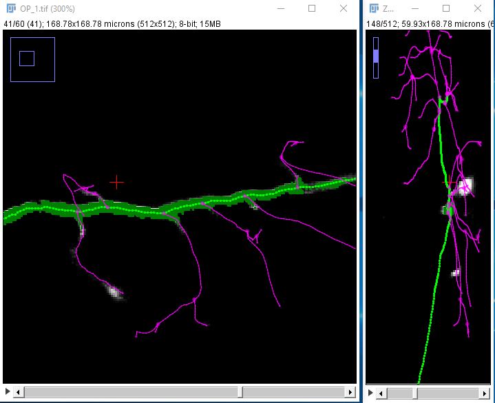
| Accurate node placement requires XY, ZY and XZ views to be visible. You can do so at startup, by making sure that Default: XY, ZY and XZ views is selected, or by clicking in Display ZY/XZ Views in the Options tab if you have already started SNT. | Error creating thumbnail: Unable to save thumbnail to destination
|
| Find the approximate location of your start point by moving your mouse in the XY window, holding down ⇧ Shift to synchronize the view in the other panes. At this point, you should enable cursor auto-snapping in the Main tab using suitable parameters for your image. | 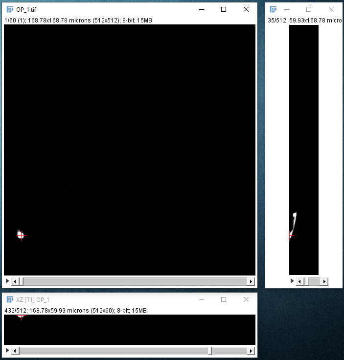
|
| When you press + to zoom in, all the panes will zoom in on the point that the crosshair is over, so each time you press +, make sure you move your mouse pointer so that it's still over the structure of interest. You may want to adjust in the Views widget (Options tab) whether all views should zoom synchronously. At this point, you should adjust a suitable snapping neighborhood both in 2D (XY) and 3D (Z). Note that when Z-snapping is enabled, all views become synchronized, |
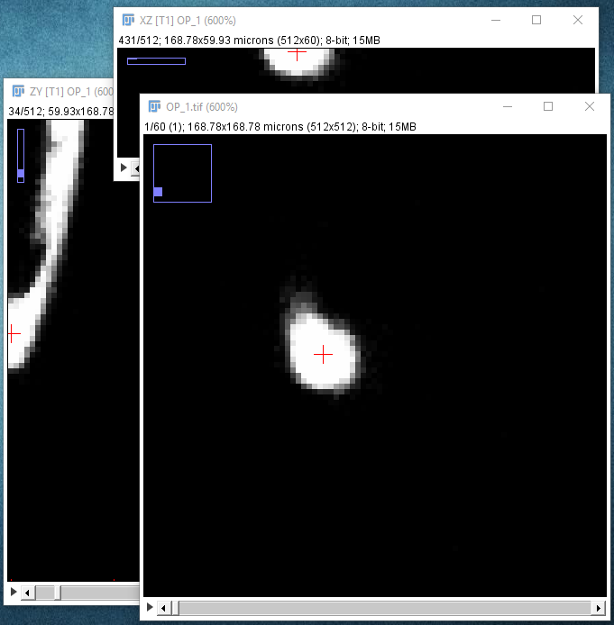
|
| Locate the center of the structure to be clicked on. If cursor auto-snapping is enabled, simply mouse over the structure, otherwise, try moving the mouse and scroll wheel in each of the panes (holding down ⇧ Shift so synchronize the views in all three panes). Note that you can toggle the cursor auto-snapping feature at will, by pressing the shortcut S. Also, note that you can "click" on the brightest voxel of a voxel column, by pressing M.
When you're happy with the point under the crosshairs, left-click to start the path: |
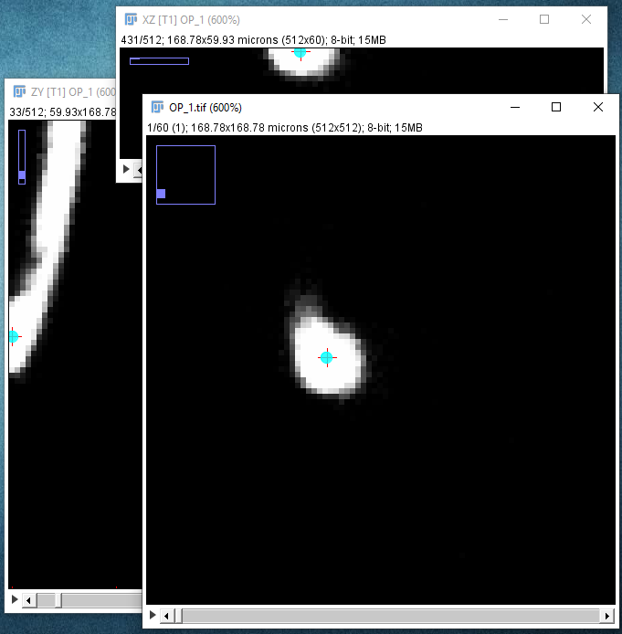
|
| Zoom out again with the - key, and similarly zoom in on the next point you want to be on your path to place it precisely: | 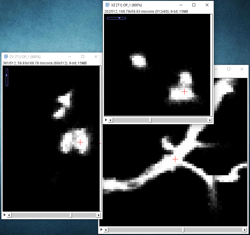
|
| The path along the neuron may not follow the center line perfectly: | 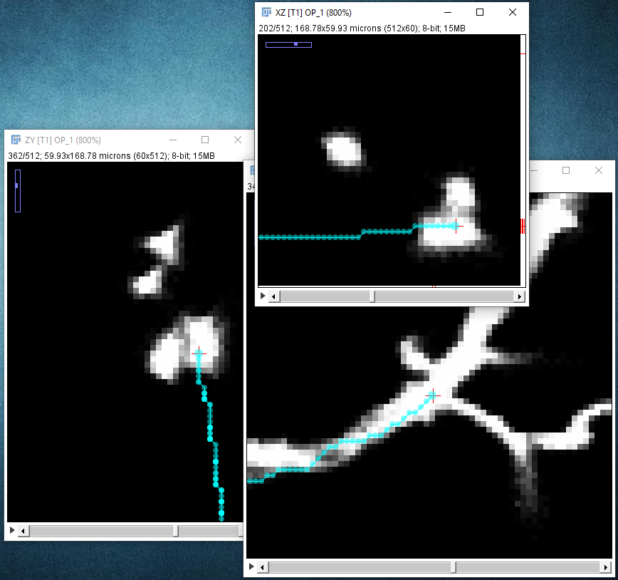
|
| ... but you can later improve that with the Refine/Fit › Fit Path... option in the Path Manager, which tries to align the path to the midline of the structure to sub-voxel accuracy: | 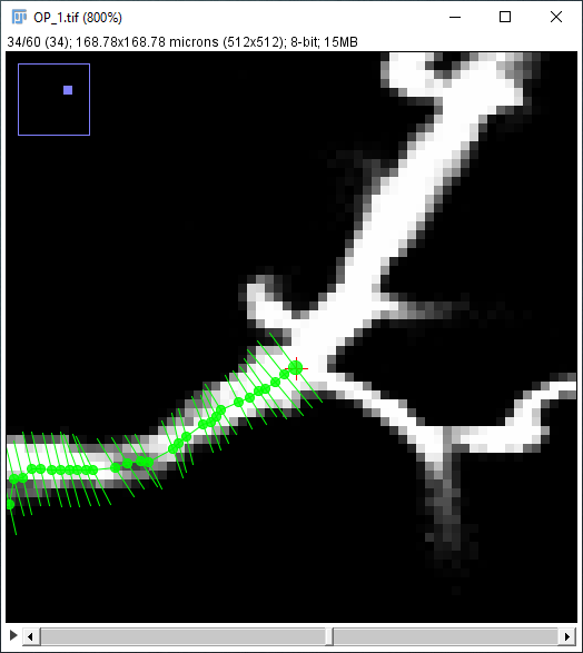
|
| Home | Manual | Walk-throughs | Screencasts | Shortcuts | Rec. Viewer | Analysis | Scripting | Modeling | FAQ |
