SNT: Scripting
| Home | Manual | Walk-throughs | Screencasts | Shortcuts | Rec. Viewer | Analysis | Scripting | Modeling | FAQ |
Contents
SNT API
The most up-to-date SNT API can be found at https://morphonets.github.io/SNT.
Script Templates
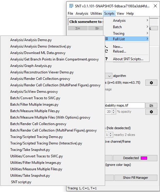
SNT comes packaged with script templates demonstrating various analysis, tracing, image processing and batch processing routines. These templates can be found both in the Scripts menu of the SNT dialog and in the Templates › Neuroanatomy menu of Fiji's Script Editor. Scripts can be written in any language supported by Fiji's Script Editor.
Analysis
- Analysis_Demo_(Interactive).py Exemplifies how to programmatically interact with a running instance of SNT to analyze traced data. Because of all the GUI updates, this approach is significantly slower than analyzing reconstructions directly (see Analysis_Demo.py for comparison)
- Analysis_Demo.py A Jython demo of how SNT can analyze neuronal reconstructions fetched from online databases such as MouseLight, NeuroMorpho or FlyCircuit.
- Download_ML_Data.groovy Exemplifies how to programmatically retrieve data from MouseLight's database at ml-neuronbrowser.janelia.org: It iterates through all the neurons in the server and downloads data (both JSON and SWC formats) for cells with soma associated with the specified Allen Reference Atlas (ARA) compartment. Downloaded files will contain all metadata associated with the cell (i.e., labeling used, strain, etc.)
- Get_Branch_Points_in_Brain_Compartment.groovy Exemplifies how to extract morphometric properties of a MouseLight cell associated with a specific brain region/neuropil compartment. Requires internet connection.
- Graph_Analysis.py Demonstrates how to handle neurons as graph structures (graph theory) in which nodes connected by edges define the morphology of the neuron. SNT represents neurons as directed graphs (assuming the root -typically the soma- as origin) and allows data be processed using the powerful jgrapht library. In this demo, the graph diameter (i.e., the length of the longest shortest path or the longest graph geodesic) of a cellular compartment is computed for a neuron fetched from the MouseLight database.
- Reconstruction_Viewer_Demo.py Exemplifies how to render reconstructions and neuropil annotations in a stand-alone Reconstruction Viewer.
- SciView_Demo.groovy Exemplifies how bridge SNT with SciView.
- Extensive_Sholl_Stats.groovy Exemplifies how to perform linear and polynomial regression on tabular Sholl data.
Boilerplate
This menu hosts script templates containing extensible boilerplate code in several programming languages, namely BeanShell, Groovy and Jython. The most essential imports and script parameters are included to facilitate rapid development.
Tracing
- Scripted_Tracing_Demo.py Exemplifies how to programmatically perform A* tracing between two points without GUI interaction, which allows for automated tracing of relatively simple structures (e.g., neurospheres neurites, microtubule bundles, etc). In this demo, points are retrieved from the SWC file of SNT's "demo tree", effectively recreating the initial SWC data.
- Scripted_Tracing_Demo_(Interactive).py Exemplifies how to programmatically interact with a running instance of SNT to perform auto-tracing tasks.
- Take_Snapshot.py Displays a WYSIWYG image of a tracing canvas. Exemplifies how to script SNT using SNTService.
Batch
This menu hosts scripts that process files in bulk. Namely:
- Convert_Traces_to_SWC.py Converts all .traces files in a directory into SWC.
- Filter_Multiple_Images.py Bulk filtering of image files using Frangi Vesselness.
- Measure_Multiple_Files.py/Measure_Multiple_Files_(With_Options).groovy Bulk measurements of reconstruction files.
- Render_Cell_Collection.groovy Exemplifies how to quickly render large collections of cells from a directory of files in Reconstruction Viewer.
- Render_Cell_Collection_(MultiPanel_Figure).groovy Exemplifies how to generate a publication-quality multi-panel figure in which multiple reconstructions are sorted and color-coded by a specified morphometric trait (e.g., cable length).
Python Notebooks
Direct access to the SNT API from the Python programming language is made possible through the pyimagej module. This enables full integration between SNT and any library in the Python ecosystem (numpy, scipy, etc.). The Notebooks directory in the SNT repository contains several examples at different complexity levels.
Here, we will exemplify basic functionality. Please refer to the complete examples for more details. Once the Python environment is properly setup, one can initialize Fiji:
import imagej
ij = imagej.init('sc.fiji:fiji', headless=False)
Then, one can use pyjnius (bundled with pyimagej) to import the needed SNT (Java) classes. E.g., to download a neuron reconstruction from the MouseLight database and calculate summary statistics on it, you would import the MouseLightLoader and TreeStatistics classes:
from jnius import autoclass
MouseLightLoader = autoclass('tracing.io.MouseLightLoader')
TreeStatistics   = autoclass('tracing.analysis.TreeStatistics')
Now you can access all the attributes and methods these classes offer. Let's get a summary of the inter-node distances for a specific mouse cortical motor neuron (ID = "AA0100" in the MouseLight database).
def run():
    loader = MouseLightLoader("AA0100")
    if not loader.isDatabaseAvailable():
        print("Could not connect to ML database", "Error")
        return
    if not loader.idExists():
        print("Somehow the specified id was not found", "Error")
        return

    a_tree = loader.getTree('axon', None) # compartment, color
    s_stats = TreeStatistics(a_tree)
    metric = TreeStatistics.INTER_NODE_DISTANCE
    summary_stats = s_stats.getSummaryStats(metric)
    s_stats.getHistogram(metric).show()
    print("The average inter-node distance is %d" % summary_stats.getMean())
Adding Scripts to SNT
There are two ways to have your own scripts appear in SNT's Scripts menu. The easiest way is to go to Scripts › New... from the SNT dialog. This command will open an instance of Fiji's Script Editor with pre-loaded boilerplate code in the scripting language of your choice. If you save the script and then choose Scripts › Reload..., your new script will appear in the full list of scripts found at Scripts › Full List....
Alternatively, you can save scripts into the "scripts" sub-directory under the main Fiji directory while including SNT in the filename (e.g., C:\Users\user\Desktop\Fiji.app\scripts\My_SNT_Script.py or /home/user/Fiji.app/scripts/My_SNT_Script.py).
Did you write a useful script? Please submit a pull request on GitHub so that it can be distributed with Fiji!
Examples
Scripting Reconstruction Viewer
Programmatic control over an open instance of Reconstruction Viewer (either called from within SNT or as a standalone application) can be achieved by selecting the Tools & Utilities › Script This Viewer... command. It will then open an instance of Fiji's script editor with a boilerplate template containing the most essential imports and script parameters. The default programming language for this template can be chosen from the drop-down menu of the Preferred Language option.
The following script exemplifies how to extend the boilerplate template to control the Viewer in real-time.
#@ Context context
#@ DatasetService ds
#@ DisplayService display
#@ ImageJ ij
#@ LegacyService ls
#@ LogService log
#@ LUTService lut
#@ SNTService snt
#@ UIService ui


"""
file:
version:
info:
"""

from sc.fiji.snt import (Path, PathAndFillManager, SNT, SNTUI, Tree)
from sc.fiji.snt.analysis import (MultiTreeColorMapper, PathProfiler, RoiConverter,
        TreeAnalyzer, TreeColorMapper, TreeStatistics)
from sc.fiji.snt.analysis.graph import GraphUtils
from sc.fiji.snt.analysis.sholl import TreeParser
from sc.fiji.snt.annotation import (AllenCompartment, AllenUtils, VFBUtils, ZBAtlasUtils)
from sc.fiji.snt.io import (FlyCircuitLoader, MouseLightLoader, NeuroMorphoLoader)
from sc.fiji.snt.plugin import (SkeletonizerCmd, StrahlerCmd)
from sc.fiji.snt.util import (BoundingBox, PointInImage, SNTColor, SWCPoint)
from sc.fiji.snt.viewer import (Annotation3D, OBJMesh, MultiViewer2D, Viewer2D, Viewer3D)

# Documentation Resources: https://imagej.net/SNT:_Scripting
# SNT API: https://morphonets.github.io/SNT
# Rec. Viewer's API: https://morphonets.github.io/SNT/index.html?sc/fiji/snt/viewer/Viewer3D.html
# Tip: Programmatic control of the Viewer's scene can be set using the Console info
# produced when calling viewer.logSceneControls() or pressing 'L' when viewer is frontmost

# If opening this template from the standalone RV, the instance ID of the Viewer (e.g., 2)
# will be automatically passed as a parameter to getRecViewer()
viewer = snt.getRecViewer()


# Added code begins here ##################################################################
import time

def do_stuff(viewer):

    viewer.logSceneControls()

    # Load a neuron from Mouse Secondary Motor Area from the MouseLight database.
    loader = MouseLightLoader("AA0100")
    if not loader.isDatabaseAvailable():
        ui.showDialog("Could not connect to ML database", "Error")
        return
    if not loader.idExists():
        ui.showDialog("Somehow the specified id was not found", "Error")
        return

    # Extract nodes with tag "axon".
    axon = loader.getTree('axon')
    # Do the same for the dendrites.
    dendrites = loader.getTree('dendrites')

    # Load the Allen CCF Mouse Reference Brain
    # and add it to the scene.
    viewer.loadRefBrain('mouse')

    # Add both Trees to the scene
    viewer.addTree(axon)
    dendrites.setColor('cyan')
    viewer.addTree(dendrites)

    # Get the OBJMesh object representing the maximum depth Allen CCF compartment
    # containing the soma point and add it to the scene.
    soma_annotation = loader.getSomaCompartment()
    viewer.addMesh(soma_annotation.getMesh())

    # Enforce side perspective.
    viewer.setViewMode('side')

    # Next, we will applying a color mapping to the axon
    # using branch order as the metric and the Ice Lut.
    # Make an instance of TreeColorMapper using SciJava context.
    mapper = TreeColorMapper(context)
    # Get the net.imglib2.display.ColorTable object.
    lut = mapper.getColorTable('Ice.lut')
    # Color code the axon and render in scene.
    # The min and max values returned by the mapper are used
    # to set the range of the color bar legend.
    bounds = viewer.colorCode(axon.getLabel(), TreeColorMapper.STRAHLER_NUMBER, lut)
    viewer.addColorBarLegend(lut, bounds[0], bounds[1])
    # Display a text annotation of the cell ID and metric used by the mapper.
    scene_annotation = "{}: Branch Order".format(axon.getLabel())
    viewer.addLabel(scene_annotation)

    # Begin a rotation animation for the objects in scene.
    viewer.setAnimationEnabled(True)
    # Wait some time before applying a new color mapping
    # based on path distances, using a different LUT (Fire).
    time.sleep(5)

    lut = mapper.getColorTable('Fire.lut')
    # Remap the axon Tree and update scene.
    bounds = viewer.colorCode(axon.getLabel(), TreeColorMapper.PATH_DISTANCE, lut)
    viewer.addColorBarLegend(lut, bounds[0], bounds[1])
    scene_annotation = "{}: Path Distance".format(axon.getLabel())
    viewer.addLabel(scene_annotation)


do_stuff(viewer)
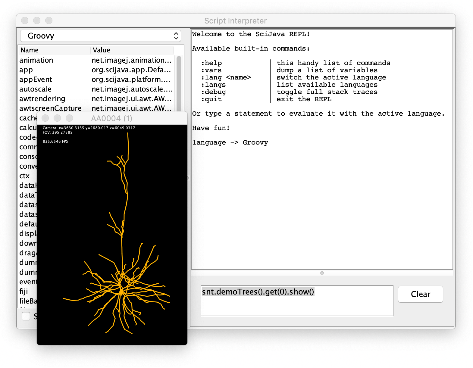
Script Interpreter
Some of SNT's functionality is accessible in the Script Interpreter. Here is an example:
| Home | Manual | Walk-throughs | Screencasts | Shortcuts | Rec. Viewer | Analysis | Scripting | Modeling | FAQ |


