ImageJ

Gaussian Convolution (Fiji/ImgLib2)
Author	Stephan Preibisch
Maintainer	Stephan Preibisch
Source	[1]
Initial release	20 December 2011
Latest version	20 December 2011
Development status	active
Website	[2]

Purpose

The gauss package for ImgLib2 is an generic, optimized implementation of the traditional Gaussian convolution. It can perform anisotropic, n-dimensional convolution on any image or any interval on an image, if required even in-place.

The computation is performed multi-threaded and accesses each pixel of the input and output containers only once to guarantee high performance, even on paged cell containers. The precision of the computation can be of any ImgLib2 NumericType, however, there are more efficient implementations for convolution with float and double precision. Any precision of gaussian convolution can be computed on any type of real valued input data, it will be internally wrapped to either float or double. For other conversions (e.g. perform a gaussian convolution on complex float data with complex double precision) respective converters need to be provided. However, any NumericType can always be convolved with its own precision. Warning: this might reduce the accuracy of the computation significantly if the Type itself is an integer type.

Documentation

The Gauss package for ImgLib2 consists of several classes which abstract the convolution operations to n dimensions. The developer/user should use the static methods provided in the Gauss.java class. It will determine itself which class should be used with which parameters in order to provide the best performance possible.

Computing gaussian convolutions on entire images

For computing a Gaussian convolution on an entire Img<T>, simply call one the following lines of code:

import net.imglib2.algorithm.gauss.Gauss;

// the source
final Img< T > img = ...

// define the sigma for each dimension
final double[] sigma = new double[ img.numDimensions() ];
for ( int d = 0; d < sigma.length; ++d )
    sigma[ d ] = 1 + d;

//
// float-precision
//
// compute with float precision, but on T
final Img< T > convolved = Gauss.inFloat( sigma, img );

// compute with float precision, and output a FloatType Img
final Img< FloatType > convolved = Gauss.toFloat( sigma, img );

// compute with float precision in-place
Gauss.inFloatInPlace( sigma, img );

//
// double-precision
//
// compute with double precision, but on T
final Img< T > convolved = Gauss.inDouble( sigma, img );

// compute with double precision, and output a FloatType Img
final Img< DoubleType > convolved = Gauss.toDouble( sigma, img );

// compute with double precision in-place
Gauss.inDoubleInPlace( sigma, img );

//
// precision defined by the type T itself (this will produce garbage if T has insufficient range 
// or accuracy like ByteType, IntType, etc, but will work nicely on for example ComplexFloatType)
//
// compute with precision of T
final Img< T > convolved = Gauss.inNumericType( sigma, img );

// compute with precision of T in-place
Gauss.inNumericTypeInPlace( sigma, img );

By default, the Gaussian convolution will use the OutOfBoundsMirrorFactory with single boundary. If another OutOfBoundsFactory is desired, it can be defined on any of those methods as follows:

// compute with float precision, but on T using an periodic (FFT-like) strategy where at the end of
// each dimension the image simply starts again
final Img< T > convolved = Gauss.inFloat( sigma, img, 
  new OutOfBoundsPeriodicFactory<FloatType, RandomAccessibleInterval<FloatType>>() ) );

Computing gaussian convolutions on RandomAccessibles with Intervals

For more advanced use of the Gaussian convolution, it accepts RandomAccessibles as input and output, too. In this way the developer has complete freedom which area to convolve and where to write the result. The input and output can be any RandomAccessible, i.e. also any kind of transformed View or Type.

To perform a Gaussian convolution on RandomAccessible you need to specify more input variables:

• the sigma in each dimension
• the input RandomAccessible (has to cover all the area required for the convolution, you might need to use Views.extend( ... ) if it is too small
• the Interval in which the Randomaccessible should be convolved. Note that more pixels around this area are required to perform the convolution, see implementation
• the output RandomAccessible specifies the target, i.e. where the result will be written to (can be the same as the input)
• the Location in the output RandomAccessible defines where the content will be inserted
• an ImageFactory for creating the temporary images, it has to be of the type in which the computation is performed. If it is inFloat, it will require an ImgFactory<FloatType>, inDouble will require ImgFactory<DoubleType> and inNumericType needs an ImageFactory<T>

An example on how to call the most generic version of the Gaussian convolution can be found below in the examples section.

Some examples

// create a new, empty 2-d image
final ArrayImgFactory<FloatType> factory = new ArrayImgFactory<FloatType>();
final Img<FloatType> img = factory.create( new int[]{ 512, 256 }, new FloatType() );

// fill it with some funny content			
int i = 0;
for ( final FloatType f : img )
	f.set( i++ );
			
for ( final FloatType f : img )
	if ( i++ % 7 == 0 || i % 8 == 0 )
		f.set( f.get() * 1.5f );

// show the input			
ImageJFunctions.show( img );

// define the 2-d sigmas
final double[] sigma = new double[] { 2, 0.75 };

// compute a gauss convolution with double precision
ImageJFunctions.show( Gauss.inDouble( sigma, img ) );	

// compute a Gaussian convolution in-place in a small Interval	
Gauss.inFloat( sigma, Views.extendMirrorSingle( img ), new FinalInterval( new long[]{300,150},
	new long[]{ 400,200 } ), img, new Location( new long[] {300,150} ), img.factory() );

// show the result
ImageJFunctions.show( img );

Another nice example of the generality of the gaussian convolution is the Game of Death 2 which uses Gaussian convolution to simulate diffusion of different species of viruses. It redefines the add() operator of our new NumericType called LifeForm which can then be used to start the simulation. The Game of Death 2 is included in the imglib repository.

Implementation

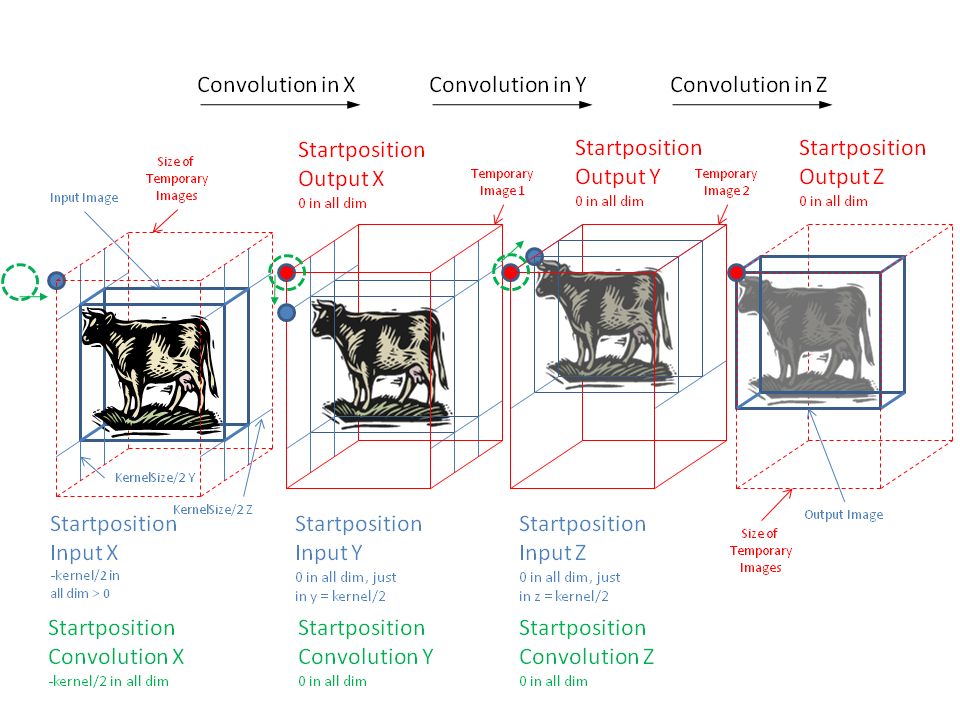
The first (obvious) core idea of the implementation is to break down the convolution into one-dimensional convolutions along each dimension. In order to properly convolve all input data, a continuously decreasing area has to be convolved when going along each dimension (see figure). This is necessary as the input for dimension d+1 has to be convolved in dimension d in order to produce the correct result.

The second core idea is to not iterate over the output but over the input to save operations and access the input as little as possible as it might be an expensive operation (page cell container, renderer, ...). Furthermore, the symmetry of the gauss kernel allows to skip almost half of all operations as each input pixel contributes left and right of itself with with the same weight. This, however, includes a more complicated logic, special cases at the beginning and end of each line, as well as different operations if the kernel is larger than the convolved image.

For more details please refer to the source code for now, it is linked on top of this page.