ImageJ

MOPS feature correspondences (example 1)

MOPS feature correspondences (example 2)

Feature Extraction SIFT/MOPS (Fiji)
Author	Stephan Saalfeld ([1])
Maintainer	Stephan Saalfeld
Source	on GitHub
Initial release	2008
Latest version	September 29th, 2009
Development status	stable, active
Category	Feature Extraction, Registration, Plugins

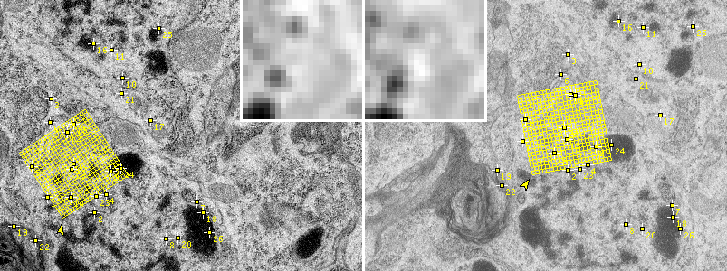
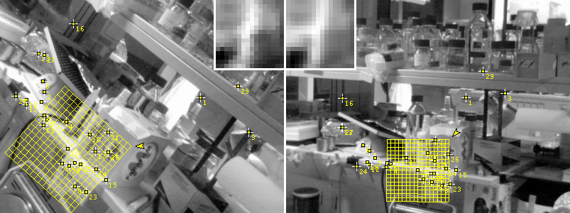
The plugins "Extract SIFT Correspondences" and "Extract MOPS Correspondences" identify a set of corresponding points of interest in two images and export them as PointRoi. Interest points are detected using the Difference of Gaussian detector thus providing similarity-invariance. Corresponding points are best matches from local feature descriptors that are consistent with respect to a common geometric transformation.

The plugins use the Scale Invariant Feature Transform (SIFT) and Multi-Scale Oriented Patches (MOPS) for local feature description. The thus established matches are filtered using the Random Sample Consensus (RANSAC).

The extracted sets of corresponding landmarks and the calculated transformations are used in TrakEM2, Register Virtual Stack Slices and BUnwarpJ for image registration.

Parameters

Error creating thumbnail: Unable to save thumbnail to destination

Scale Invariant Interest Point Detector

initial gaussian blur

Accurate localization of keypoints requires initial smoothing of the image. If your images are blurred already, you might lower the initial blur σ₀ slightly to get more but eventually less stable keypoints. Increasing σ₀ increases the computational cost for Gaussian blur, setting it to σ₀=3.2px is equivalent to keep σ₀=1.6px and use half maximum image size. Tip: Keep the default value σ₀=1.6px as suggested by Lowe (2004).

steps per scale octave

Keypoint candidates are extracted at all scales between maximum image size and minimum image size. This Scale Space is represented in octaves each covering a fixed number of discrete scale steps from σ₀ to 2σ₀. More steps result in more but eventually less stable keypoint candidates. Tip: Keep 3 as suggested by Lowe (2004) and do not use more than 10.

minimum image size

The Scale Space stops if the size of the octave would be smaller than minimum image size. Tip: Increase the minimum size to discard large features (i.e. those extracted from looking at an image from far, such as the overall shape).

maximum image size

The Scale Space starts with the first octave equal or smaller than the maximum image size. Tip: By reducing the size, fine scaled features will be discarded. Increasing the size beyond that of the actual images has no effect.

upscale image first

Create the first scale octave with double the size of the original image in order to find features at the original pixel resolution. Tip: Do this only for very small images and if you desperately need more features.

Feature Descriptor

Interest points are matched using a local descriptor. Corresponding interest points have typically very similar local descriptors.

feature descriptor size

The SIFT-descriptor consists of n×n gradient histograms, each from a 4×4px block. n is this value. Lowe (2004) uses n=4. We found larger descriptors with n=8 perform better for Transmission Electron Micrographs from serial sections.

The MOPS-descriptor is simply a n×n intensity patch with normalized intensities. Brown (2005) suggests n=8. We found larger descriptors with n>16 perform better for Transmission Electron Micrographs from serial sections.

feature descriptor orientation bins

For SIFT-descriptors, this is the number of orientation bins b per 4×4px block as described above. Tip: Keep the default value b=8 as suggested by Lowe (2004).

closest/ next closest ratio

Correspondence candidates from local descriptor matching are accepted only if the Euclidean distance to the nearest neighbour is significantly smaller than that to the next nearest neighbour. Lowe (2004) suggests a ratio of r=0.8 which requires some increase when matching things that appear significantly distorted.

Geometric Consensus Filter

maximal alignment error

Matching local descriptors gives many false positives, but true positives are consistent with respect to a common transformation while false positives are not. This consistent set and the underlying transformation are identified using RANSAC. This value is the maximal allowed transfer error of a match to be counted as a good one. Tip: Set this to about 10% of the image size.

minimal inlier ratio

The ratio of the number of true matches to the number of all matches including both true and false used by RANSAC. 0.05 means that minimally 5% of all matches are expected to be good while 0.9 requires that 90% of the matches were good. Only transformations with this minimal ratio of true consent matches are accepted. Tip: Do not go below 0.05 (and only if 5% is more than about 7 matches) except with a very small maximal alignment error to avoid wrong solutions.

expected transformation

The expected underlying transformation between both images. Tip: For serial section microscopy images, this is typically a rigid transformation.

Legal Notice

This software embodies methods for which the following patents have been issued:

1. "Method and apparatus for identifying scale invariant features in an image and use of same for locating an object in an image", David G. Lowe, US Patent 6,711,293 (March 23, 2004). Asignee: The University of British Columbia.
2. "Multi-image feature matching using multi-scale oriented patches", Matthew Brown, Richard Szeliski, US Patent 7,382,897 (June 3, 2008). Asignee: Microsoft Corporation.

References

1. Lowe, David G. (2004). "Distinctive Image Features from Scale-Invariant Keypoints". International Journal of Computer Vision 60 (2): 91–110. doi:10.1023/B:VISI.0000029664.99615.94.
2. Brown, Matthew; Szeliski, Richard; Winder, Simon (2005). "Multi-Image Matching Using Multi-Scale Oriented Patches". Proceedings of the 2005 IEEE Computer Society Conference on Computer Vision and Pattern Recognition (CVPR'05) Volume 1: 510–517. doi:10.1109/CVPR.2005.235.
3. Fischler, Martin A.; Bolles, Robert C. (1981). "Random sample consensus: a paradigm for model fitting with applications to image analysis and automated cartography". Communications of the ACM 24 (6): 381–395. doi:10.1145/358669.358692